CAB403 Study Guide | 2023 Semester 1
Timothy Chappell | Notes for CAB403 at the Queensland University of Technology
Unit Description
Disclaimer
Everything written here is based off the QUT course content and the recommended text books. If any member of the QUT staff or a representative of such finds any issue with these guides please contact me at jeynesbrook@gmail.com.
Week 1
Operating Systems
What is an Operating System
An operating system is a program that acts as an intermediary between a user of a computer and the computer hardware. It's acts as a resource allocator managing all resources and decides between conflicting requests for efficient and fair resource use. An OS also controls the execution of programs to prevent errors and improper use of the computer.
The operating system is responsible for:
- Executing programs
- Make solving user problems easier
- Make the computer system convenient to use
- Use the computer hardware in an efficient manner
Computer System Structure
Computer systems can be divided into four main components
- Hardware: These items provide basic computing resources, i.e. CPU, memory, I/O devices.
- Operating system: Controls and coordinates the use of hardware among various applications and users.
- Application programs: These items define the ways in which the system resources are used to solve the computing problems of the use, i.e. word processors, compilers, web browsers, database systems, video games.
- Users: People, machines, or other computers.
Computer Startup
A bootstrap program is loaded at power-up or reboot. This program is typically stored in ROM or EPROM and is generally know as firmware. This bootstrap program is responsible for initialising all aspects of the system, loading the operating system kernel, and starting execution.
Computer System Organisation
- I/O devices and the CPU can execute concurrently.
- Each device controller is in charge of a particular device type and has a local buffer.
- The CPU moves data from/to the main memory to/from local buffers.
- I/O is from the device to the local buffer of a particular controller.
- The device controller informs the CPU that it has finished its operation by causing an interrupt.
Common Functions of Interrupts
Operating systems are interrupt driven. Interrupts transfer control to the interrupt service routine. This generally happens through the interrupt vector which contains the addresses of all the service routines. The interrupt architecture must save the address of the interrupted instruction.
A trap or exception is a software-generated interrupt caused by either an error or a user request.
Interrupt Handling
The operating systems preserves the state of the CPU by storing registers and the program counter. It then determines which type of interrupt occured, polling or vectored interrupt system.
Once determined what caused the interrupt, separate segments of code determine what action should be taken for each type of interrupt.
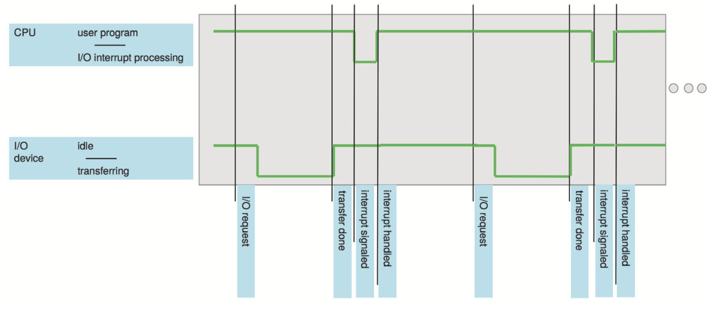
Figure: Interrupt timeline for a single program doing output.
I/O Structure
There are two ways I/O is usually structured:
- After I/O starts, control returns to the user program only upon I/O completion.
- Wait instructions idle the CPU until the next interrupt.
- At most, one I/O request is outstanding at a time. This means no simultaneous I/O processing.
- After I/O starts, control returns to the user program without waiting for I/O
completion.
- System call: Request to the OS to allow users to wait for I/O completion.
- A device-status table containes entries for each I/O device indicating its type, address, and state.
- The OS indexes into the I/O device table to determine the device status and to modify a table entry to include an interrupt.
Storage Definitions and Notation Review
The basic unit of computer storage is a bit. A bit contains one of two values, 0 and 1. A byte is 8 bits, and on most computers is the smallest convenient chunck of storage.
- A kilobyte, or KB, is \(1,024\) bytes
- A megabyte, or MB, is \(1,024^2\) bytes
- A gigabyte, or GB, is \(1,024^3\) bytes
- A terabyte, or TB, is \(1,024^4\) bytes
- A petabyte, or PB, is \(1,024^5\) bytes
Direct Memory Access Structure
This method is used for high-speed I/O devices able to transmit information at close to memory speeds. Device controllers transfer blocks of data from buffer storage directly to main memory without CPU intervention. This means only one interrupt is generated per block rather than the one interrupt per byte.
Storage Structure
- Main memory: Only large storage media that the CPU can access directly.
- Random access
- Typically volatile
- Secondary storage: An extension of main memory that provides large non-volatile storage capacity.
- Magnetic discs: Rigid metal or glass platters covered with magnetic recording material. The disk surface is logically divided into tracks which are sub-diveded into sectors. The disk controller determines the logical interaction between the device and the computer.
- Solid-state disks: Achieves faster speeds than magnetic disks and non-volatile storage capacity through various technologies.
Storage Hierarchy
Storages systems are organised into a hierarchy:
- Speeds
- Cost
- Volatility.
There is a device driver for each device controller used to manage I/O. They provide uniform interfaces between controllers and the kernel.
Caching
Caching allows information to be copied into a faster storage system. The main memory can be viewed as a cache for the secondary storage.
Faster storage (cache) is checked first to determine if the information is there:
- If so, information is used directly from the cache
- If not, data is copied to the cache and used there
The cache is usually smaller and more expensive that the storage being cached. This means cache management is an important design problem.
Computer-System Architecture
Most systems use a single general-purpose processor. However, most systems have special-purpose processors as well.
Multi-processor systems, also known as parallel systems or tightly-coupled systems, usually come in two types; Asymmetric Multi-processing or Symmetric Multi-processor. Multi-processor systems have a few advantages over a single general-purpose processor:
- Increase throughput
- Economy of scale
- Increased reliability, i.e. graceful degradation or fault tolerance
Clustered Systems
Clustered systems are like Multi-processor systems, they have multiple systems working together.
- These systems typically share storage via a storage-area network (SAN).
- Provide a high-availability service which survices failures:
- Asymmetric clustering have one machine in hot-standby mode.
- Symmetric clustering have multiple nodes running applications, monitoring each other.
- Some clusters are for high-performance computing (HPC). Applications running on these clusters must be written to use parallelisation.
- Some have a distributed lock manager (DLM) to avoid conflicting operations.
Operating System Structure
Multi-programming organises jobs (code and data) so the CPU always has one to execute. This is needed for efficiency as a single user cannot keep a CPU and I/O devices busy at all times. Multi-programming works by keeping a subset of total jobs in the system, in memory. One job is selected and run via job scheduling. When it has to wait (for I/O for example), the OS will switch to another job.
Timesharing is a logical extension in which the CPU switches jobs so frequently that users can interact with each job while it is running.
- The response time should be less than one second.
- Each user has at least one program executing in memory (process).
- If processes don't fit in memory, swapping moves them in and out to run.
- Virtual memory allows execution of processes not completely in memory.
- If several jobs are ready to run at the same time, the CPU scheduler handles which to run.
Operating-System Operations
Dual-mode operations (user mode and kernel mode) allow the OS to protect itself and other system components. A mode bit provided by the hardware provides the ability to distinguish when a system is running user code or kernel code. Some instructions are designated as privileged and are only executable in kernel mode. System calls are used to change the mode to kernel, a return from call resets the mode back to user.
Most CPUs also support multi-mode operations, i.e. virtual machine manages (VMM) mode for guest VMs.
Input and Output
printf()
printf() is an output function included in stdio.h. It outputs a character
stream to the standard output file, also known as stdout, which is normally
connected to the screen.
It takes 1 or more arguments with the first being called the control string.
Format specifications can be used to interpolate values within the string. A
format specification is a string that begins with % and ends with a conversion
character. In the above example, the format specifications %s and %d were used.
Characters in the control string that are not part of a format specification are
placed directly in the output stream; characters in the control string that are
format specifications are replaced with the value of the corresponding argument.
Example 1: Output with printf()
printf("name: %s, age: %d\n", "John", 24); // "name: John, age: 24"
scanf()
scanf() is an input function included in stdio.h. It reads a series of characters
from the standard input file, also known as stdin, which is normally connected
to the keyboard.
It takes 1 or more arguments with the first being called the control string.
Example 2: Reading input with scanf()
char a, b, c, s[100];
int n;
double x;

scanf("%c%c%c%d%s%lf", &a, &b, &c, &n, n, &x);
Relevant Links
Pointers
A pointer is a variable used to store a memory address. They can be used to access memory and manipulate an address.
Example 1: Various ways of declaring a pointer
// type *variable;

int *a;
int *b = 0;
int *c = NULL;
int *d = (int *) 1307;

int e = 3;
int *f = &e; // `f` is a pointer to the memory address of `e`
Example 2: Dereferencing pointers
int a = 3;
int *b = &a;

printf("Values: %d == %d\nAddresses: %p == %p\n", *b, a, b, &a);
Relevant Links
Functions
A function construct in C is used to write code that solves a (small) problem.
A procedural C program is made up of one or more functions, one of them being
main(). A C program will always begin execution with main().
Function parameters can be passed into a function in one of two ways; pass by value and pass by reference. When a parameter is passed in via value, the data for the parameters are copied. This means any changes to said variables within the function will not affect the original values passed in. Pass by reference on the other hand passes in the memory address of each variable into the function. This means that changes to the variables within the function will affect the original variables.
Example 1: Function control
#include <stdio.h>

void prn_message(const int k);

int main(void) {
    int n;

    printf("There is a message for you.\n");
    printf("How many times do you want to see it?\n");

    scanf("%d", &n);

    prn_message(n);

    return 0;
}

void prn_message(const int k) {
    printf("Here is the message:\n");

    for (size_t i = 0; i < k; i++) {
        printf("Have a nice day!\n");
    }
}
Example 2: Pass by values
#include <stdio.h>

void swapx(int a, int b);

int main(void) {
    int a = 10;
    int b = 20;

    // Pass by value
    swapx(a, b);

    printf("within caller - a: %d, b: %b\n", a, b); // "within caller - a: 10, b: 20"

    return 0;
}

void swapx(int a, int b) {
    int temp;

    temp = a;
    a = b;
    b = temp;

    printf("within function - a: %d, b: %b\n", a, b); // "within function - a: 20, b: 10"
}
Example 3: Pass by value
#include <stdio.h>

void swapx(int *a, int *b);

int main(void) {
    int a = 10;
    int b = 20;

    // Pass by reference
    swapx(&a, &b);

    printf("within caller - a: %d, b: %b\n", a, b); // "within caller - a: 20, b: 10"

    return 0;
}

void swapx(int *a, int *b) {
    int temp;

    temp = *a;
    *a = *b;
    *b = temp;

    printf("within function - a: %d, b: %b\n", *a, *b); // "within function - a: 20, b: 10"
}
Example 4: Function pointers
#include <stdio.h>

void function_a(int num) {
    printf("Function A: %d\n", num);
}

void function_b(int num) {
    printf("Function B: %d\n", num);
}

void caller(void (*function) (int)) {
    function(1);
    function(2);
    function(3);
}

int main(void) {
    caller(function_a);
    caller(function_b);

    return 0;
}
Week 2
Operating System Structures
Operating System Services
Operating systems provide an environment for execution of programs and services to programs and users.
There are many operating system services that provide functions that are helpful to the user such as:
- User interface: Almost all operating systems have a user interface. This can be in the form of a graphical user interface (GUI) or a command-line (CLI).
- Program execution: The system must be able to load a program into memory and run that program, end execution, either normally or abnormally.
- I/O operations: A running program may require I/O, which may involve a file or an I/O device.
- File-system manipulation: The file system is of particular interest. Programs need to read and write files and directories, create and delete them, search them, list file information, manage permissions, and more.
- Communication: Processors may exchange information, on the same computer or between computers over a network.
- Error detection: OS needs to be constantly aware of possible errors:
- May occur in the CPU and memory hardware, in I/O devices, in user programs, and more.
- For each type of error, the OS should take the appropriate action to ensure correct and consistent computing.
- Debugging facilities can greatly enhance the user's and programmer's abilities to efficiently use the system.
Another set of OS functions exist for ensuring the efficient operation of the system itself via resource sharing.
- Resource allocation: When multiple users or multiple jobs are running concurrently, resources must be allocated to each of them.
- Accounting: To keep track of which users use how much and what kinds of resources.
- Protection and security: The owners of information stored in a multi-user
or networked computer system may want to control use of that information. Concurrent
processes should not interfere with each other.
- Protection involves ensuring that all access to system resources is controlled.
- Security of the system from outsiders requires user authentication. This also extends to defending external I/O devices from invalid access attempts.
- If a system is to be protected and secure, pre-cautions must be instituted throughout it. A chain is only as strong as its weakest link.
System Calls
System calls provide an interface to the services made available by an operating system. These calls are generally written in higher-level languages such as C and C++. These system calls however, are mostly accessed by programs via a high-level application programming interface (API) rather than direct system call use.
The three most common APIs are Win32 API for Windows, POSIX API for POSIX-based systems, and JAVA API for the Java virtual machine (JVM)
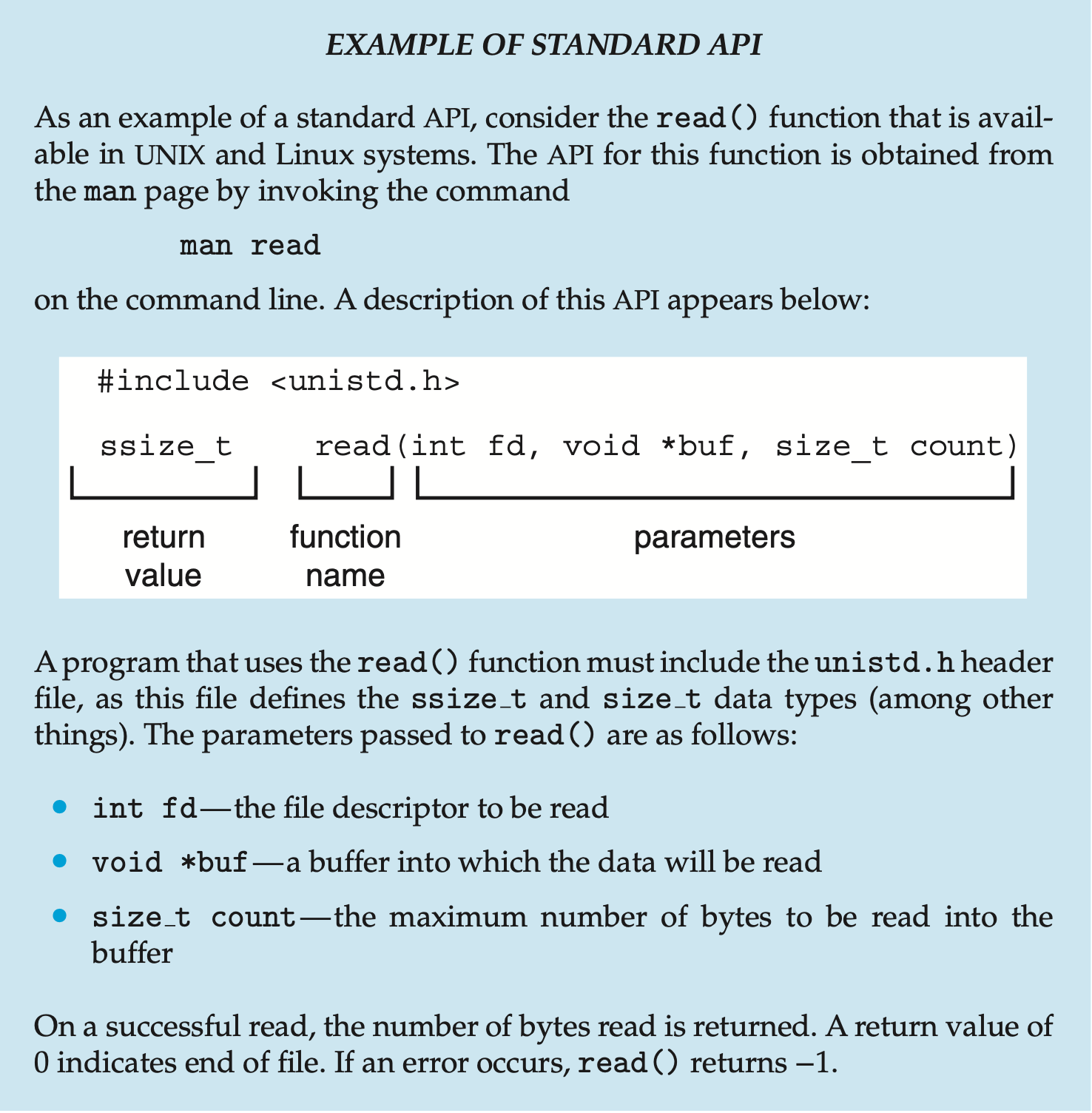
Typically, a number is associated with each system call. The system-call interface maintains a table indexed according to these numbers. The system call interface invokes the intended system call in the OS kernel and returns a status of the systema call and any return values. The caller needs to know nothing about how the system call is implemented, it just needs to obey the API and understand what the OS will do as a result call.
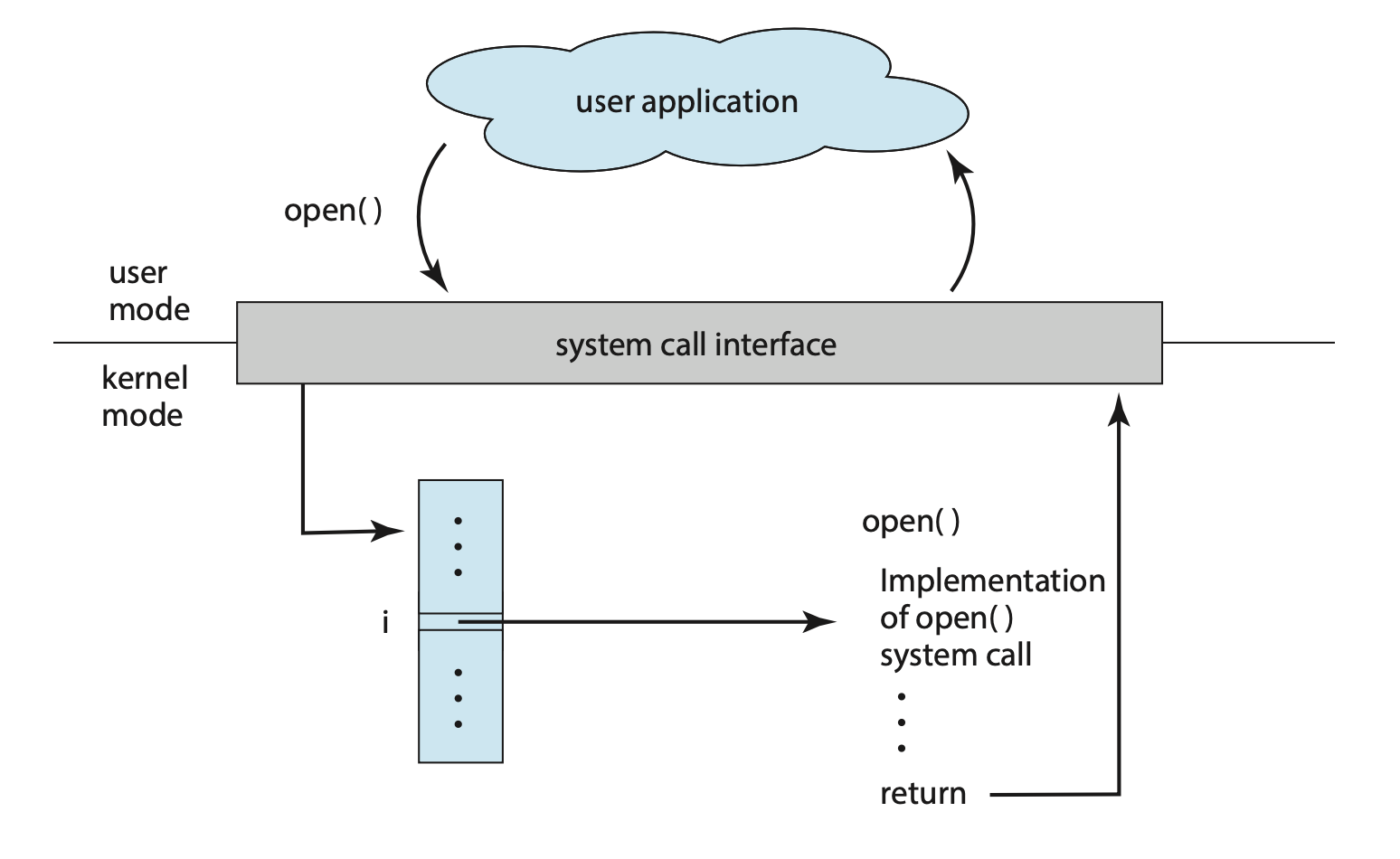 Figure: The handling of a user application invoking the
 open() system call.
There are many types of system calls:
- Process control
- File management
- Device management
- Information maintenance
- Communications
- Protection
Often, more information is required than simply the identity of the system call. There are three general methods used to pass parameters to the OS:
- Pass parameters into registers. This won't always work however as there may be more parameters than registers.
- Store parameters in a block, or table, in memory, and pass the address of the block as a parameter in a register.
- Parameters are placed, or pushed, onto the stack by the program and popped off the stack by the operating system. This method does not limit the number length of the parameters being passed.
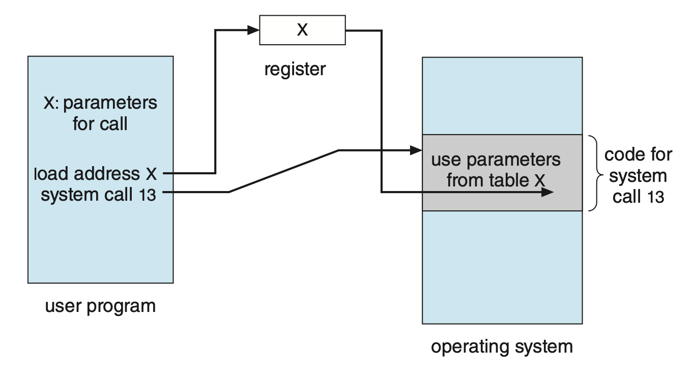 Figure: Passing of parameters as a table.
System Programs
System programs provide a convenient environment for program development and execution. They can be generally divided into:
- File manipulation
- Status information sometimes stored in a file modification
- Programming language support
- Program loading and execution
- Communications
- Background services
- Application programs
UNIX
UNIX is limited by hardware functionality. The original UNIX operating system had limited structing. The UNIX OS consists of two separable parts:
- Systems programs
- The kernel:
- Consists of everything below the system-call interface and above the physical hardware.
- Provides the file system, CPU scheduling, memory management, and other operating-system functions.
Operating System Structure
There are a few ways to organise an operating system.
Layered
The operating system is divided into a number of layers, each built on top of the lower layers. The bottom layer (layer 0), is the hardware; the highest is the user interface.
Due to the modularity, layers are selected such that each uses functions and services of only lower-level layers.
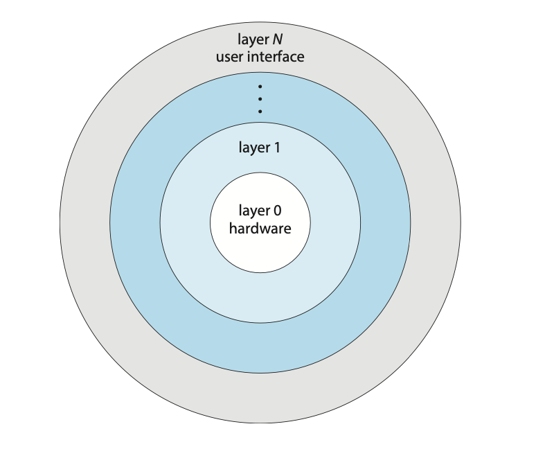 Figure: A layered operating system.
Microkernel System
In this organisation method, as much as possible is moved from the kernel into user space. An example OS that uses a microkernel is Mach, which parts of the MacOSX kernel (Darwin) is based upon. Communication takes place between user modules via message passing.
| Advantages | Disadvantages |
|---|---|
| Easier to extend a microkernel | Performance overhead of user space to kernel space communication |
| Easier to port the operating system to new architectures | |
| More reliable (less code is running in kernel mode) | |
| More secure |
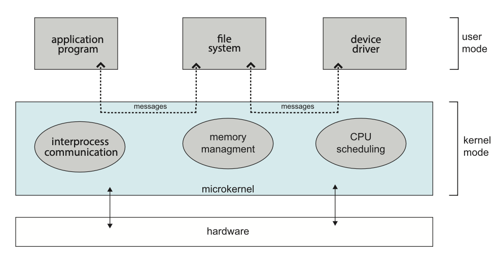 Figure: Architecture of a typical microkernel.
Hybrid System
Most modern operating systems don't use a single model but a use concepts from a variety. Hybrid systems combine multiple approaches to address performance, security, and usability needs.
For example, Linux is monolithic, because having the operating system in a single address space provides very efficient performance. However, it's also modular, so that new functionality can be dynamically added to the kernel.
Modules
Most modern operating systems implement loadable kernel modules (LKMs). Here, the kernel has a set of core components and can link in additional services via modules, either at boot time or during run time
Each core component is separate, can talk to others via known interfaces, and is loadable as needed within the kernel.
Arrays
An array is a contiguous sequence of data items of the same type. An array name is an address, or constant pointer value, to the first element in said array.
Aggregate operations on an array are not valid in C, this means that you cannot
assign an array to another array. To copy an array you must either copy it component-wise
(typically via a loop) or via the memcpy() function in string.h.
Example 1: Arrays in practice
#include <stdio.h>

const int N = 5;

int main(void) {
    // Allocate space for a[0] to a[4]
    int a[N];
    int i;
    int sum = 0;

    // Fill the array
    for (i = 0; i < N; i++) {
        a[i] = 7 + i * i;
    }

    // Print the array
    for (i = 0; i < N; i++) {
        printf("a[%d] = %d\n", i, a[i]);
    }

    // Sum the elements
    for (i = 0; i < N; i++) {
        sum += a[i];
    }

    printf("\nsum = %d\n", sum);

    return 0;
}
Example 2: Arrays and Pointers
#include <stdio.h>

const int N = 5;

int main(void) {
    int a[N];
    int sum;
    int *p;

    // The following two calls are the same
    p = a;
    p = &a[0];

    // The following two calls are the same
    p = a + 1;
    p = &a[1];


    // Version 1
    sum = 0;

    for (int i = 0; i < N; i++) {
        sum += a[i];
    }

    // Version 2
    sum = 0;

    for (int i = 0; i < N; i++) {
        sum += *(a + i);
    }
}
Example 3: Bubble Sort
#include <stdio.h>

void swap(int *arr, int i, int j);
void bubble_sort(int *arr, int n);

void main(void) {
    int arr[] = { 5, 1, 4, 2, 8 };
    int N = sizeof(arr) / sizeof(int);

    bubble_sort(arr, N);

    for (int i = 0; i < N; i++) {
        printf("%d: %d\n", i, arr[i]);
    }

    return 0;
}

void swap(int *arr, int i, int j) {
    int temp = arr[i];
    arr[i] = arr[j];
    arr[j] = temp;
}

void bubble_sort(int *arr, int n) {
    for (int i = 0; i < n - 1; i++) {
        for (int j = 0; j < n - 1; j++) {
            if (arr[j] > arr[j + 1]) {
                swap(arr, j, j + 1);
            }
        }
    }
}
Example 4: Copying an Array
#include <stdio.h>
#include <string.h>

int main(void) {
    // Copying an array component-wise
    int array_one[5] = { 1, 2, 3, 4, 5 };
    int array_two[5];

    for (int idx = 0; idx < 5; idx++) {
        array_two[idx] = array_one[idx];
    }

    // Copying an array via memcpy
    memcpy(array_two, array_one, sizeof(int) * 5);
}
Relevant Links
Strings
A string is a one-dimensional array of type char. All strings must end with a
null character \0 which is a byte used to represent the end of a string.
A character in a string can be accessed either by an element in an array of by making use of a pointer.
Example 1: Strings in practice
char *first = "john";
char last[6];

last[0] = 's';
last[1] = 'm';
last[2] = 'i';
last[3] = 't';
last[4] = 'h';
last[5] = '\0';

printf("Name: %s, len: %lu", first, strlen(first));
Relevant Links
Structures
Structures are named collections of data which are able to be of varying types.
Example 1: Structures in practice
struct student {
    char *last_name;
    int student_id;
    char grade;
};

// By using `typedef` we can avoid prefixing the type with `struct`
typedef struct unit {
    char *code;
    char *name;
} unit;

void update_student(struct student *student);
void update_grade(unit *unit);

int main(void) {
    struct student s1 = {
        .last_name = "smith",
        .student_id = 119493029,
        .grade = 'B',
    };

    s1.grade = 'A';

    update_student(&s1);


    unit new_unit;

    new_unit.name = "Microprocessors and Digital Systems";

    update_unit(&new_unit);
}

void update_student(struct student *student) {
    // `->` shorthand for dereference of struct
    student->last_name = "doe";
    student->grade = 'C';
}

void update_unit(unit *unit) {
    // `->` shorthand for dereference of struct
    unit->code = "CAB403";
    unit->name = "Systems Programming";
}
Relevant Links
Dynamic Memory Management
Memory in a C program can be divided into four categories:
- Code memory
- Static data memory
- Runtime stack memory
- Heap memory
Code Memory
Code memory is used to store machine instructions. As a program runs, machine instructions are read from memory and executed.
Static Data Memory
Static data memory is used to store static data. There are two categories of static data: global and static variables.
Global variables are variables defined outside the scope of any function as
can be seen in example 1. Static variables on the other hand are defined with
the static modifier as seen in example 2.
Both global and static variables have one value attached to them; they are
assigned memory once; and they are initialised before main begins execution
and will continue to exist until the end of execution.
Example 1: Global variables.
int counter = 0;

int increment(void) {
    counter++;

    return counter;
}
Example 2: Static variables.
int increment(void) {
    // will be initialised once
    static int counter = 0;

    // increments every time the function is called
    counter++;

    return counter;
}
Runtime Stack Memory
Runtime stack memory is used by function calls and is FILO (First in, Last out). When a function is invoked, a block of memory is allocated by the runtime stack to store the information about the function call. This block of memory is termed as an Activation Record.
The information about the function call includes:
- Return address.
- Internal registers and other machine-specific information.
- Parameters.
- Local variables.
Heap Memory
Heap memory is memory that is allocated during the runtime of the program. On many systems, the heap is allocated in an opposite direction to the stack and grows towards the stack as more is allocated. On simple systems without memory protection, this can cause the heap and stack to collide if too much memory is allocated to either one.
To deal with this, C provides two functions in the standard library to handle
dynamic memory allocation; calloc() (contiguous allocation) and malloc()
(memory allocation).
void *calloc(size_t n, size_t s) returns a pointer to enough space in memory
to store n objects, each of s bytes. The storage set aside is automatically
initialised to zero.
void *malloc(size_t s) returns a pointer to a space of size s and leaves the
memory uninitialised.
Example 3: malloc() and calloc()
#include <stdio.h>
#include <stdlib.h>

int main() {
    int num_of_elements;
    int *ptr;
    int sum = 0;

    printf("Enter number of elements: ");
    scanf("%d", &num_of_elements);

    ptr = malloc(num_of_elements * sizeof(int));
    // or
    // ptr = calloc(num_of_elements, sizeof(int));

    if (ptr == NULL) {
        printf("[Error] - Memory was unable to be allocated.");

        exit(0);
    }

    printf("Enter elements: ");

    for (int i = 0; i < n; i++) {
        scanf("%d", ptr + i);

        sum += *(ptr + i);
    }

    printf("Sum = %d", sum);

    free(ptr);

    return 0;
}
Relevant Links
Week 3
Processes
An operating system executes a variety of programes either via:
- Batch systems (jobs)
- or Time-shared systems (user programs or tasks)
A process, sometimes referred to as a job, is simply a program in execution. The status of the current activity of a process is represented by the value of the program counter and the contents of the processor’s registers.
A process is made up of multiple parts:
- Text section: The executable code
- Data section: Global variables
- Heap section: Memory that is dynamically allocated during program run time
- Stack section: Temporary data storage when invoking functions (such as function parameters, return addresses, and local variables)
It's important to note that a program itself is not a process but rather a passive entity. In contrast, a process is an active entity, with a program counter specifying the next instruction to execute and a set of associated resources.
As a process executes, it changes state. A process may be in one of the following states:
- new: The process is being created.
- running: Instructions are being executed.
- waiting: The process is waiting for some event to occur.
- ready: The process is waiting to be assigned to a processor.
- terminated: The process has finished execution.
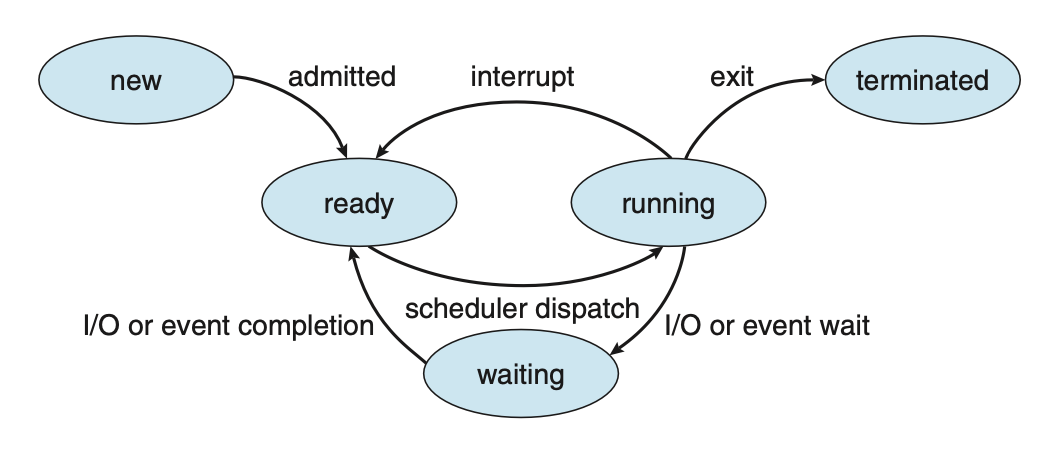 Figure: Diagram of process state.
Process Control Block (PCB)
Each process is represented in the OS by a process control block, also known as a task control block. It contains information associated with a specific process such as:
- Process state: The state of the process.
- Program counter: The address of the next instruction to be executed for this process.
- CPU registers: The contents of all process-centric registers. Along with the program counter, this state information must be saved when an interrupt occurs, to allow the process to be continued correctly afterward when it is rescheduled to run.
- CPU scheduling information: Information about process priority, pointers to scheduling queues, and any other scheduling parameters.
- Memory-management information: This information may include such items as the value of the base and limit registers and the page tables, or the segment tables, depending on the memory system used by the operating system.
- Accounting information: This information includes the amount of CPU and real time used, time limits, account numbers, job or process numbers, etc..
- I/O status information: This information includes the list of I/O devices allocated to the process, a list of open files, etc..
Threads
In a single-threaded model, only a single thread of instructions can be executed. This means only a single tasks can be completed at any given time. For example, in a word document, the user cannot simultaneously type in characters and run the spell checker.
In most modern operating systems however, the use of multiple threads allows more than one task to be performed at any given moment. A multithreaded word processor could, for example, assign one thread to manage user input while another thread runs the spell checker.
In a multi-threaded system, the PCB is expanded to include information for each thread.
Process Scheduling
The objective of multi-programming is to have some process running at all times so as to maximize CPU utilization. A process scheduler is used to determine which process should be executed. The number of processes currently in memory is known as the degree of multiprogramming
When a process enters the system, it's put into a ready queue where it then waits to be executed. When a process is allocated a CPU core for execution it executes for a while and eventually terminates, is interrupted, or waits for the occurrence of a particular event. Any process waiting for an event to occur gets placed into a wait queue.
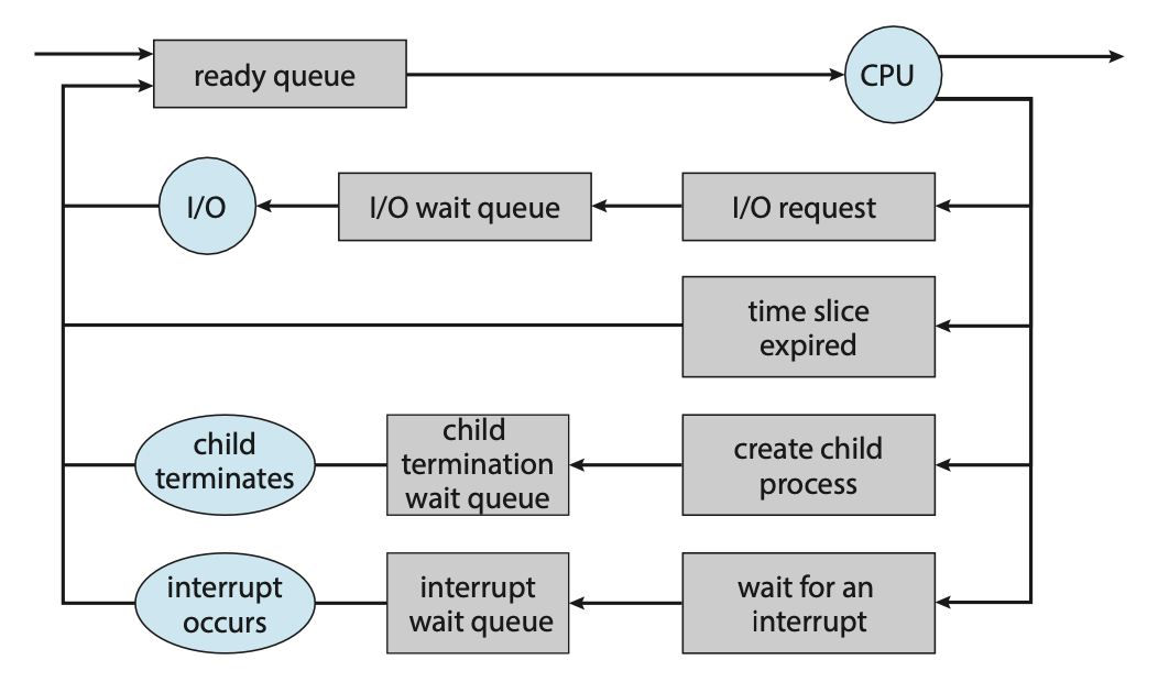 Figure: Queueing-diagram representation of process scheduling.
Most processos can be described as either:
- I/O bound: A I/O bound process that spends more of its time doing I/O operations.
- CPU bound: Spends more of its time doing more calculations with infrequent I/O requests.
Context Switch
Interrupts cause the operating system to change a CPU core from its current task and to run a kernel routine. These operations happen frequently so it's important to ensure that when returning to the process, no information was lost.
Switching the CPU core to another process requires performing a state save of the current process and a state restore of a different process. This task is known as a context switch. When a context switch occurs, the kernel saves the context of the old process in its PCB and loads the saved context of the new process scheduled to run.
The time between a context switch is considered as overhead as no useful work is done while switching. The more complex the OS and PCB, the longer it takes to context switch.
Process Creation
During execution, a process may need to create more processes. The creating process is called a parent process, and the new processes are called the children of that process. Each of these new processes may in turn create other processes, forming a tree of processes. Processes are identified by their process identifier (PID).
When a process is created, it will generally require some amount of resources to accomplish its task. A child process may be able to obtain its resources directly from the operating system, or it may be constrained to a subset of the resources of the parent process.
When a process creates a new process, two possibilities for execution exist:
- The parent continues to execute concurrently with its children.
- The parent waits until some or all of its children have terminated.
There are also two address-space possibilities for the new process:
- The child process is a duplicate of the parent process (it has the same program and data as the parent).
- The child process has a new program loaded into it.
A new process is created by the fork() system call. The new process consists
of a copy of the address space of the original process. The return code for the
fork() is zero for the new (child) process, whereas the (nonzero) process identifier
of the child is returned to the parent.
Once forked, it's typical for exec() to be called on one of the two processes.
The exec() system call loads a binary file into memory (destroying the memory
image of the program containing the exec() system call) and starts its execution.
For example, this code forks a new process and, using execlp(), a version of
the exec() system call, overlays the process address space with the UNIX command
/bin/ls (used to get a directory listing).
#include <sys/types.h>
#include <sys/wait.h>
#include <stdio.h>
#include <unistd.h>

int main() {
    pid_t pid;
    /* fork a child process */
    pid = fork();

    if (pid < 0) { /* error occurred */
        fprintf(stderr, "Fork failed\n");

        return 1;
    } else if (pid == 0) { /* child process */
        execlp("/bin/ls", "ls", NULL);
    } else { /* parent process */
        /* parent will wait for the child to complete */
        wait(NULL);

        printf("Child complete\n");
    }

    return 0;
}
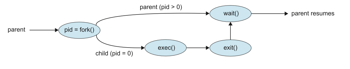 Figure: Process creation using the fork() system call.
Process Termination
A process terminates when it finishes executing its final statement and asks the
operating system to delete it by using the exit() system call. At that point,
the process may return a status value (typically an integer) to its waiting parent
process (via the wait() system call).
A parent may terminate the execution of one of its children for a variety of reasons, such as:
- The child has exceeded its usage of some of the resources that it has been allocated.
- The task assigned to the child is no longer required.
- The parent is exiting, and the operating system does not allow a child to continue if its parent terminates.
A parent process may wait for the termination of a child process by using the
wait() system call. The wait() system call is passed a parameter that allows
the parent to obtain the exit status of the child. This system call also returns
the process identifier of the terminated child so that the parent can tell which
of its children has terminated:
pid t pid;
int status;

pid = wait(&status);
When a process terminates, its resources are deallocated by the operating system.
However, its entry in the process table must remain there until the parent calls
wait(), because the process table contains the process’s exit status.
If a child process is terminated but the parent has not called wait(), the process
is known as a zombie process. If a parent is terminated before calling wait(), the process
is know as an orphan.
Interprocess Communication
Processes within a system may be independent or cooperating. A process is cooperating if it can affect or be affected by the other processes executing in the system.
There are a variety of reasons for providing an environment that allows process cooperation:
- Information sharing
- Computational speedup
- Modularity
- Convenience
Cooperating processes require an interprocess communication (IPC) mechanism that will allow them to exchange data. There are two fundamental models of interprocess communication: shared memory and message passing.
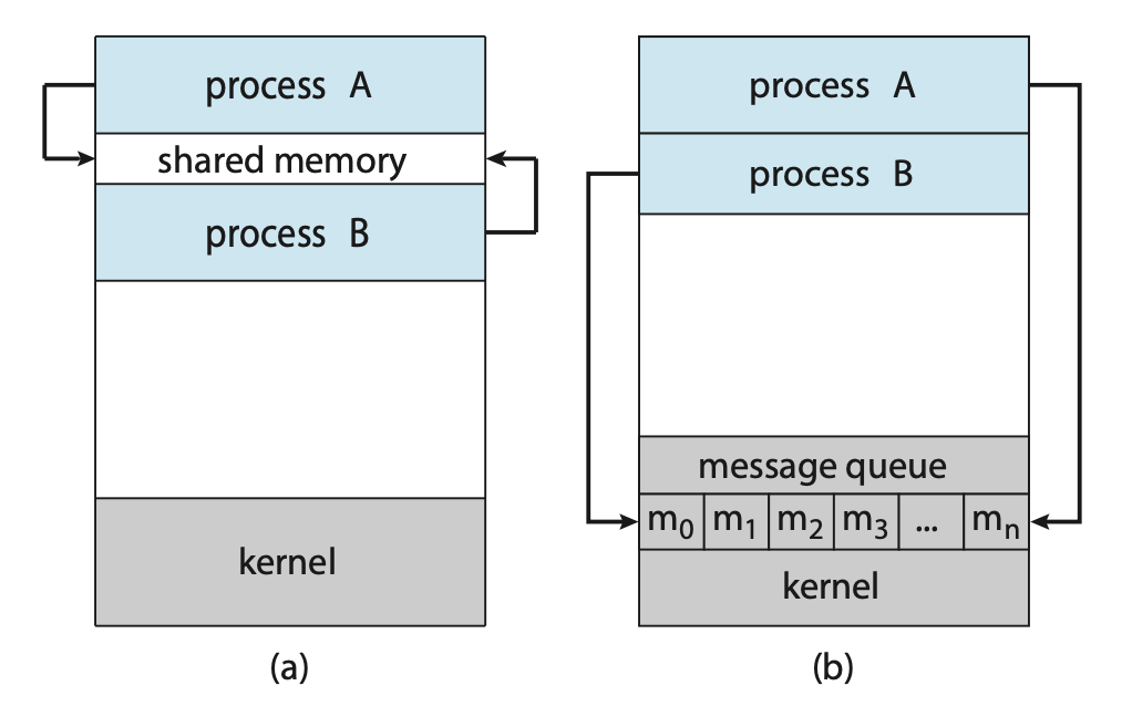 Figure: Communications models. (a) Shared memory. (b) Message passing.
In the shared-memory model, a region of memory that is shared by the cooperating processes is established. Processes can then exchange information by reading and writing data to the shared region. In the message-passing model, communication takes place by means of messages exchanged between the cooperating processes.
Producer-Consumer Problem
The Producer-Consumer problem is a common paradigm for cooperating processes. A producer process produces information that is consumed by a consumer process.
One solution to the producer–consumer problem uses shared memory. To allow producer and consumer processes to run concurrently, we must have available a buffer of items that can be filled by the producer and emptied by the consumer. This buffer will reside in a region of memory that is shared by the producer and consumer processes.
Two types of buffers can be used. The unbounded buffer places no practical limit on the size of the buffer. The consumer may have to wait for new items, but the producer can always produce new items. The bounded buffer assumes a fixed buffer size. In this case, the consumer must wait if the buffer is empty, and the producer must wait if the buffer is full.
Message Passing
Message passing provides a mechanism to allow processes to communicate and to synchronize their actions without sharing the same address space.
A message-passing facility provides at least two operations:
send(message)receive(message)
Before two processes can communicate, they first need to establish a communication link.
This could be via physical hardware:
- Shared memory.
- Hardware bus.
or logical:
- Direct or indirect communication.
- Synchronous or asynchronous communication.
- Automatic or explicit buffering.
Direct Communication
Under direct communication, each process that wants to communicate must explicitly name the recipient or sender of the communication.
send(P, message)- send a message to process P.receive(Q, message)- receive a message from process Q.
A communication link in this scheme has the following properties:
- A link is established automatically.
- The processes need to know only each other’s identity to communicate.
- A link is associated with exactly two processes.
- Between each pair of processes, there exists exactly one link.
Indirect Communication
With indirect communication, the messages are sent to and received from mailboxes, or ports. A mailbox can be viewed abstractly as an object into which messages can be placed by processes and from which messages can be removed. Each mailbox has a unique identification.
send(A, message)— Send a message to mailbox A.receive(A, message)— Receive a message from mailbox A.
The operating system then must provide a mechanism that allows a process to do the following:
- Create a new mail box.
- Send and receive messages through the mailbox.
- Delete a mail box.
In this scheme, a communication link has the following properties:
- A link is established between a pair of processes only if both members of the pair have a shared mailbox.
- A link may be associated with more than two processes.
- Between each pair of communicating processes, a number of different links may exist, with each link corresponding to one mailbox.
Now suppose that processes \(P_1\), \(P_2\), and \(P_3\) all share mailbox A.
Process \(P_1\) sends a message to A, while both \(P_2\) and \(P_3\) execute
a receive() from A. Which process will receive the message sent by \(P_3\)?
The answer depends on which of the following methods we choose:
- Allow a link to be associated with at most two processes
- Allow only one process at a time to execute a receive operation
- Allow the system to select arbitrarily the receiver. Sender is notified who the receiver was.
Synchronisation
Communication between processes takes place through calls to send() and receive()
primitives. Message passing may be either blocking or nonblocking also known as
synchronous and asynchronous.
- Blocking send: The sending process is blocked until the message is received by the receiving process or by the mailbox.
- Nonblocking send: The sending process sends the message and resumes operation.
- Blocking receive: The receiver blocks until a message is available.
- Nonblocking receive: The receiver retrieves either a valid message or a null.
Different combinations of send() and receive() are possible. When both send()
and receive() are blocking, we have a rendezvous between the sender and the
receiver.
Buffering
Whether communication is direct or indirect, messages exchanged by communicating processes reside in a temporary queue. These queues can be implemented in three ways:
- Zero capacity: The queue has a maximum length of zero; thus, the link cannot have any messages waiting in it. In this case, the sender must block until the recipient receives the message.
- Bounded capacity: The queue has finite length \(n\); thus, at most \(n\) messages can reside in it. If the queue is not full when a new message is sent, the message is placed in the queue (either the message is copied or a pointer to the message is kept), and the sender can continue execution without waiting. The link’s capacity is finite, however. If the link is full, the sender must block until space is available in the queue.
- Unbounded capacity: The queue’s length is potentially infinite; thus, any number of messages can wait in it. The sender never blocks.
Week 4
Threads
A thread is a basic unit of CPU utilisation. A thread consists of:
- A thread ID
- A program counter PC
- A register set
- A stack
A thread shares it's code section, data section, and other operating-system resources with others threads within the same process. A traditional process usually consists of a single thread of control, this is called a single-threaded process. A process with multiple threads of control can therefore perform more than one task at any given moment, this is called a multi-threaded process.
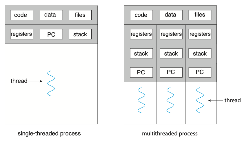 Figure: Single-threaded and multithreaded processes.
Most programs that run on modern computers and mobile devices are multithreaded. For example, A word processor may have a thread for displaying graphics, another thread for responding to keystrokes from the user, and a third thread for performing spelling and grammar checking in the background.
In certain situations, a single application may be required to perform several tasks at any one time. For example, a web server needs to accept many client requests concurently. A solution to this is to have the server run a single process that accepts requests. When a request is recieved, a new process is created to service the request. Before threads became popular, this was the most common way to handle such situation.
The problem with this however is that processes are expensive to create. If the new process will perform the same tasks as the existing process, why incur the overhead of creating another. If a web server is multithreaded, the server will create a separate thread that listens for client requests. When a new requests comes in, the server will create a new thread to service the requests and resume listening for more requests.
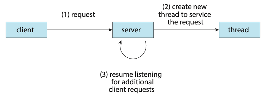 Figure: Multithreaded server architecture.
Most operating system kernels are also typically multithreaded. During system boot time on Linux systems, several kernel threads are created to handle tasks such as managing devices, memory management, and interrupt handling.
There are many benefits to using a multithreaded programming approach:
- Responsiveness: Multithreading an interactive application may allow a program to continue running even if part of it is blocked or is performing a lengthy operation.
- Resouce sharing: Processes can share resources only through techniques such as shared memory and message passing. However, threads share the memory and the resources of the process to which they belong by default.
- Economy: Allocating memory and resources for process creation is costly. Because threads share the resources of the process to which they belong, it is more economical to create and context-switch threads.
- Scalability: The benefits of multithreading can be even greater in a multiprocessor architecture, where threads may be running in parallel on different processing cores.
Multicore Programming
Due to the need for more computing performance, single-CPU systems evolved into multi-CPU systems. A trend in system design was to place multiple computing cores on a single processing chip where each core would then appear as a separate CPU to the operating system, such systems are referred to as multicore systems.
Imagine an application with four threads. On a system with a single computing core, concurrency merely means that the execution of the threads will be interleaved over time due to the processing core only being capable of executing a single thread at a time.
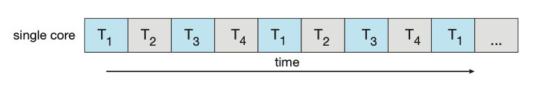 Figure: Concurrent execution on a single-core system.
On a system with multiple cores, concurrency means that some threads can run in parallel due to the system being capable of assigning a separate thread to each core.
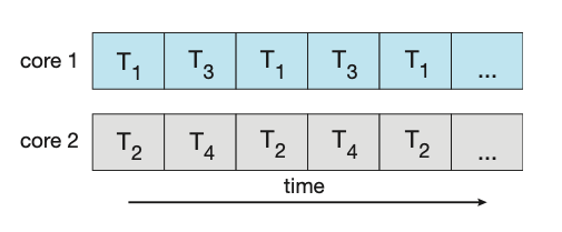
Figure: Parallel execution on a multicore system.
Types of Parallelism
There are two types of parallelism:
- Data parallelism: Focuses on distributing subsets of the same data across multiple computing cores and performing the same operation on each core.
- Task parallelism: Involves distributing not data but tasks (threads) across multiple computing cores. Each thread is performing a unique operation. Diferent threads may be operating on the same data, or they may be operating on different data.
It's important to note that these two methods are not mutually exclusive and an application may use a hybrid method of both strategies.
Multithreading Models
Support for threads may be provided either at the user level (user threads) or by the kernel (kernel threads). User threads are supported above the kernel and are managed without kenel support. Kernel threads on the other hand are supported and managed directly by the operating system.
There are three common relationships between user threads and kernel threads.
- Many-to-One Model: The many-to-one model maps many user-level threads to one kernel thread. Thread management is done by the thread library in user space, so it is efficient. However, the entire process will block if a thread makes a blocking system call. Also, because only one thread can access the kernel at a time, multiple threads are unable to run in parallel on multicore systems.
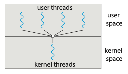
Figure: Many-to-one model.
- One-to-One Model: The one-to-one model maps each user thread to a kernel thread. It provides more concurrency than the many-to-one model by allowing another thread to run when a thread makes a blocking system call. It also allows multiple threads to run in parallel on multiprocessors. The only drawback to this model is that creating a user thread requires creating the corresponding kernel thread, and a large number of kernel threads may burden the performance of a system.
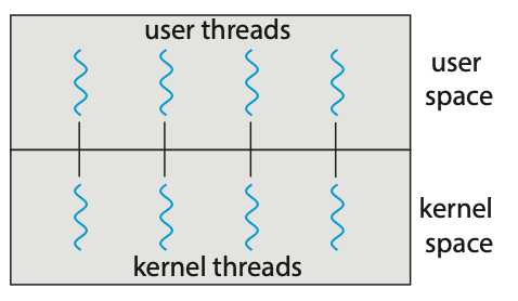
Figure: One-to-one model.
- Many-to-Many Model: The many-to-many model (Figure 4.9) multiplexes many user-level threads to a smaller or equal number of kernel threads. Although the many-to-many model appears to be the most flexible of the models discussed, in practice it is difficult to implement.
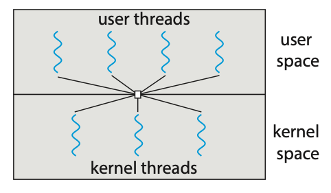
Figure: Many-to-many model.
Creating Threads
There are two general strategies forr creating multiple threads:
- Asynchronous threading: Once the parent creates a child thread, the parent resumes its execution, so that the parent and child execute concurrently and independently of one another.
- Synchronous threading: The parent thread creates one or more children and then must wait for all of its children to terminate before it resumes. Here, the threads created by the parent perform work concurrently, but the parent cannot continue until this work has been completed. Once each thread has finished its work, it terminates and joins with its parent. Only after all of the children have joined can the parent resume execution.
Pthreads
Pthreads refers to the POSIX standard (IEEE 1003.1c) defining an API fo thread creation and synchronisation. It's important to know that Pthreads is simply a specification for thread behaviour and not an implementation, that is left up to the operating-system designers.
Below is an example application using Ptheads to calculate the summation of a non-negative integer in a separate thread.
#include <pthread.h>
#include <stdio.h>
#include <stdlib.h>

int sum; // The data shared among the threads.
void *runner(void *param); // The function called by each thread.

int main(int argc, char *argv[]) {
    pthread_t tid; // The thread identifier.
    pthread_attr_t attr; // Set of thread attributes.

    // Set the default attributes of the thread.
    pthread_attr_init(&attr);

    // Create the thread.
    pthread_create(&tid, &attr, runner, argv[1]);

    // Wait for the thead to finish executing.
    pthead_join(tid, NULL);

    printf("Sum: %d\n", sum);
}

void *runner(void *param) {
    int upper = atoi(param);
    int sum = 0;

    for (int i = 1; i <= upper; i++) {
        sum += 1;
    }

    pthread_exit(0);
}
This example program creates only a single thread. With the growing dominance of
multicore systems, writing programs containing several threads has become increasingly
common. A simple method for waiting on several threads using the pthread_join()
function is to enclose the operation within a simple for loop.
#define NUM_THREADS 10

pthread_t workers[NUM_THREADS];

for (int i = 0; i < NUM_THREADS; i++) {
    pthread_join(workers[i], NULL);
}
Thread Pools
The idea behing a thread pool is to create a number of threads at start-up and place them into a pool where they sit and wait for work. In the context of a web server, when a request is recieved, rather than creating a new thread, it instead submits the request to the thread pool and resumes waiting for additional requests. Once the thread completes its service, it returns to the pool and awaits more work.
A thread pool has many benefits such as:
- Servicing a equest within an existing thead is often faster than waiting to create a new thread.
- A thread pool limits the number of threads that exist at any one point. This ensures that the system does not get overwhelmed when creating more threads than it can handle.
- Separating the task to be performed from the mechanics of creating the task allows us to use different strategies for running the task. For example, the task could be scheduled to execute after a time delay or to execute periodically.
The number of threads in the pool can be set heuristically based on factors such as the number of CPUs in the system, amount of physical memory, and the expected number of concurrent client requests. More sophisticated thread pool architectures are able to dynamically adjust the number of threads in the pool based off usage patterns.
Fork Join
The fork-join method is one in which when the main parent thread creates one or more child threads and then waits for the children to terminate and join with it.
This synchronous model is often characterised as explicit thread creation, but it is also an excellent candidate for implicit threading. In the latter situation, threads are not constructed directly during the fork stage; rather, parallel tasks are designated. A library manages the number of threads that are created and is also responsible for assigning tasks to threads.
Threading Issues
- The
fork()andexec()system calls - Signal handling
- Thread cancellation
- Thread-local storage
- Scheduler activations
Week 5
Synchronisation
A cooperating process is one that can affect or be affected by other processes executing in the system. Cooperating processes can either directly share a logical address space or be allowed to share data through shared memory or message passing. Concurrent access to shared data may result in data inconsistency.
A race condition occurs when several processes access and manipulate the same data concurrently and the outcome of the execution depends on the particular order in which the access takes place.
The Critical-Section Problem
Consider a system of \(n\) processes. Each proces has a segment of code, called the critical section, in which the process may be accessing - and updating - data that is shared with at least one other process. When one process is executing in its critical section, no other process is allowed to execute in its critical section. The critical-section problem is to design a protocol that the processes can use to synchronise their activity so as to cooperatively share data.
Each process must request permission to enter its critical section. The code implementing this request is the entry section. The critical section may be followed by an exit section. The remaining code is the remainder section.
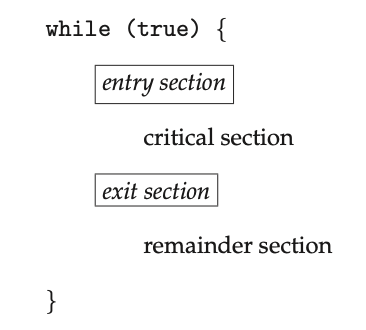
Figure: General structure of a typical process.
A solution to the critical-section problem must satisfy the following three requirements:
- Mutual exclusion: If process \(P_i\) is executing in its critical section, then no other process can be executing in their critical sections.
- Progress: If no process is executing in its critical section and some processes wish to enter their critical sections, then only those processes that are not executing in their remainder sections can participate in deciding which will enter its critical section next, and this selection cannot be postponed indefinitely.
- Bounded waiting: There exists a bound, or limit, on the number of times that other processes are allowed to enter their critical sections after a process has made a request to enter its critical section and before that request is granted.
There are two general approaches used to handle critical sections in operating systems:
- Preemptive kernels: A preemptive kernel allows a process to be preemped while it's running in kernel mode.
- Non-preemptive kernels: A non-preemptive kernel does not allow a process running in kernel mode to be preempted; A kernel-mode process will run until it exits kernel mode, blocks, or voluntarily yields control of the CPU.
A non-preemptive kernel is essentially free from race conditions on kernel data structures as only one process is active in the kernel at a time. Preemptive kernels on the other hand are not and must be carefully designed to ensure that shared kernel data is free from race conditions.
Despite this, preemptive kernels are still preferred as:
- They allow a real-time process to preempt a process currently running in kernel mode
- They are more responsive since there is less risk that a kernel-mode process will run for an arbitrarily long period before relinquishing the processor to waiting processes.
Peterson's Solution
Peterson's solution is a software-based solution to the critical-section problem. Due to how modern computer architectures perform basic machine-language instructions, there are no guarantees that Peterson's solution will work correctly on such architectures.
int turn;
boolean flag[2];

while (true) {
    flag[i] = true;
    turn = j;

    while (flag[j] && turn == j);

    // Critical section

    flag[i] = false;

    // Remainder section
}
Hardware Support for Synchronisation
Memory Barriers
How a computer architecture determines what memory guarantees it will provide to an application program is known as its memory model. A memory model falls into one of two categories:
- Strongly ordered: Where a memory modification on one processor is immediately visible to all other processors.
- Weakly ordered: Where modifications to memory on one processor may not be. immediately visible to other processors.
Memory models vary by processor type, so kernel developers cannot make assumptions regarding the visibility of modifications to memory on a shared-memory multiprocessor. To address this issue, computer architectures provide instructions that can force any changes in memory to be propagated to all other processors. Such instructions are know as memory barriers or memory fences.
When a memory barrier instruction is performed, the system ensures that all loads and stores are completed before any subsequent load or store operations are performed. This ensures that even if instructions were re-ordered, the store operations are completed in memory and visible to other processors before future load or store operations are performed.
Memory barriers are considered very low-level operations are are typically only used by kernel developers when writing specialised code that ensures mutual exclusion.
Hardware Instructions
Many computer systems provide special hardware instructions that allow us either
to test and modify the content of a word or to swap the contents of two words
atomically - that is, as one uninterruptible unit. These special instructions
can be used to solve the critical-section problem. Such examples of these instructions
are test_and_set() and
compare_and_swap.
boolean test_and_set(boolean *target) {
    boolean rv = *target;
    *target = true;

    return rv;
}
Figure: The definition of the atomic test_and_set() instruction.
int compare_and_swap(int *value, int expected, int new_value) {
    int temp = *value;

    if (*value == expected) {
        *value = new_value;
    }

    return temp;
}
Figure: The definition of the atomic compare_and_swap() instruction.
Atomic Variables
An atomic variable provides atomic operations on basic data types such as integers
and booleans. Most systems that support atomic variables provide special atomic
data types as well as functions for acessing and manipulating atomic variables.
These functions are often implemented using compare_and_swap() operations.
For example, the following increments the atomic integer sequence:
increment(&sequence);
where the increment() function is implemented using the CAS instruction:
void increment(atomic_int *v) {
    int temp;

    do {
        temp = *v;
    } while (temp != compare_and_swap(v, temp, temp + 1));
}
It's important to note however that although atomic variables provide atomic updates, they do not entirely solve race conditions in all circumstances.
Mutex Locks
Mutex, short for mutual exclusion, locks are used to protect critical sections and thus prevent race conditions. They act as high-level software tools to solve critical-section problems.
A process must first acquire a lock before entering a critical section; it then
releases the lock when it exits the critical section. The acquire() function
acquires the lock, and the release() function releases the lock. A mutex lock
has a boolean variable available whose value indicates if the lock is available
or not. Calls to either acquire() or release() must be performed atomically.
acquire() {
    while (!available); /* busy wait */
    available = false;;
}

release() {
    available = true;
}
The type of mutex lock described above is also called a spin-lock due to the
process "spinning" while waiting for the lock to become available. The main
disadvantage with spin locks is that they require busy waiting. While a process
is in its critical section, any other process that tries to entir its critical
section must loop continuously in the call to acquire(). This wastes CPU cycles
that some other process might be able to use productively. On the other hand,
spinlocks do have an advantage in that no context switch is required when a process
must wait on a lock.
Semaphores
A semaphore \(S\) is an integer variable that, apart from initialisation, is
accessed only through two standard atomic operations: wait() and signal().
Operating systems often distinguish between counting and binary semaphores. The value of a counting semaphore can range over an unrestricted domain. The value of a binary semaphore can range only between 0 and 1.
Counting semaphores can be used to control access to a given resource consisting
of a finite number of instances. The semaphore is initialised to a number of
resources available. Each process that wishes to use a resource performs a wait()
operation on the semaphore (decrementing the count). When a process releases
resource, it performs a signal() operation (incrementing the count). When the
count for the semaphore goes to 0, all resources are being used. Processes wishing
to use a resource will block until the count becomes greater than 0.
wait(S) {
    while (S <= 0); // busy wait
    S--;
}

signal (S) {
    S++;
}
Figure: Semaphore with busy waiting.
It's important to note that some definitions of the wait() and signal()
semaphore operations, like the example above, present the same problem that
spinlocks do, busy waiting. To overcome this, other definition of these functions
are modified as to when a process executes wait(), it suspends itself rather
than busy waiting. Suspending the process puts it back a waiting queue associated
with the semaphore. Control is then transferred to the CPU scheduler, which selects
another process to execute. A process that is suspended, waiting on a semaphore
\(S\), should be restarted when some other process executes a signal() operation.
A process that is suspended can be restarted by a wakeup() operation which
changes the process from the waiting state to the ready state subsequently placing
it into the ready queue.
typedef struct{
    int value;
    struct process *list;
} semaphore;

wait(semaphore *S) {
    S->value--;

    if (S->value < 0) {
        add this process to S->list;
        block();
    }
}

signal(semaphore *S) {
    S->value++;

    if (S->value <= 0) {
        remove a process P from S->list;
        wakeup(P);
    }
}
Figure: Semaphore without busy waiting.
Monitors
An abstract data type - or ADT - encapsulates data with a set of functions to operate on that data that are independent of any specific implementation of the ADT. A monitor type is an ADT that includes a set of programmer-defined operations that are provided with mutual exclusion within the monitor. The monitor type also declares the variables whose values define the state of an instance of that type, along with the bodies of functions that operate on those variables.
The representation of a monitor type cannot be used directly by the various processes. Thus, a function defined within a monitor can access only those variables declared locally within the monitor and its formal parameters. Similarly, the local variables of a monitor can be accessed by only the local functions.
The monitor construct ensures that only one process at a time is active within
the monitor. Consequently, the programmer does not need to code this synchronization
constraint explicitly. In some instances however, we need to define additional
synchronization mechanisms. These mechanisms are provided by the condition
construct. A programmer who needs to write a tailor-made synchronization scheme
can define one or more variables of type condition. The only operations that can
be invoked on a condition variable are wait() and signal().
The wait() means that the process invoking this operation is suspended until
another process invokes whereas the signal() operation resumes exactly one
suspended process. If no process is suspended, then the signal() operation has
no effect. Contrast this operation with the signal() operation associated with
semaphores, which always affects the state of the semaphore.
Now suppose that, when the x.signal() operation is invoked by a process \(P\),
there exists a suspended process \(Q\) associated with condition x. Clearly,
if the suspended process \(Q\) is allowed to resume its execution, the signaling
process \(P\) must wait. Otherwise, both \(P\) and \(Q\) would be active
simultaneously within the monitor. Two possibilities exist:
- Signal and wait: \(P\) either waits until \(Q\) leaves the monitor or waits for another condition.
- Signal and continue: \(Q\) either waits until \(P\) leaves the monitor or waits for another condition.
Liveness
Liveness refers to a set of properties that a system must satisfy to ensure that processes make progress during their execution life cycle. A process waiting indefinitely is an example of a "liveness failure". There are many different forms of liveness failure; however, all are generally characterised by poor performance and responsiveness.
Deadlock
The implementation of a semaphore with a waiting queue may result in a situation where two or more processes are waiting indefinitely for an event that can be caused only by one of the waiting processes. When such a state is reached, these processes are said to be deadlocked.
Priority Inversion
A scheduling challenge arises when a higher-priority process needs to read or modify kernel data that are currently being accessed by a lower-priority process — or a chain of lower-priority processes. Since kernel data are typically protected with a lock, the higher-priority process will have to wait for a lower-priority one to finish with the resource. The situation becomes more complicated if the lower-priority process is preempted in favor of another process with a higher priority.
This liveness problem is known as priority inversion, and it can occur only in systems with more than two priorities. Typically, priority inversion is avoided by implementing a priority-inheritance protocol. According to this protocol, all processes that are accessing resources needed by a higher-priority process inherit the higher priority until they are finished with the resources in question. When they are finished, their priorities revert to their original values.
Synchronisation Examples
Bounded-Buffer Problem
In this problem, the producer and consumer processes share the following data structures.
int n;
semaphore mutex = 1;
semaphore empty = n;
semaphore full = 0;
We assume that the pool consits of n buffers, each capable of holding one item.
The mutex binary semaphore provides mutual exclusion for accesses to the buffer
pool and is initialised to the value 1. The empty and full semaphores count
the number of empty and full buffers.
while (true) {
    // ...
    // Produce an item in next_produced
    // ...

    wait(empty);
    wait(mutex);

    // ...
    // Add next_produced to the buffer
    // ...

    signal(mutex);
    signal(full);
}
Figure: The structure of the producer process.
while (true) {
    wait(full);
    wait(mutex);

    // ...
    // Remove an item from the buffer to next_consumed
    // ...

    signal(mutex);
    signal(empty);

    // ...
    // consume the item in next_consumed
    // ...
}
Figure: The structure of the consumer process.
We can interpret this code as the producer producing full buffers for the consumer or as the consumer producing empty buffers for the producer.
Readers-Writers Problem
Suppose that the database is to be shared among several concurrent processes. Some of these processes may want only to read the database (readers), whereas others may want to update the database (writers). Two readers can access the shared data simultaneously with no adverse effects however, if a writer and some other process (either reader or writer) access the data simultaneously, chaos may ensure.
To avoid these situations from arising, it's required that the writers have exclusive access to the shared database while writing to the database. This synchronisation problem is referred to as the readers-writers problem. This problem has several variations, all involving priorities.
The first readers-writers problem requires that no reader be kept waiting unless a writer has already obtained permission to use the shared object. No reader should wait for other readers to finish simply because a writer is waiting. The second readers-writers problem requires that once a writer is ready, that writer peform its write as soon as possible. If a writer is waiting to access the object, no new readers may start reading.
A solution to either may result in starvation. In the first case, writers may starve, in the second case, readers may starve. It's because of this that other variants of the problem have been proposed.
In the following solution to the first readers-writers problem, the reader processes share the following data structures:
semaphore rw_mutex = 1;
semaphore mutex = 1;
int read_count = 0;
The semaphore rw_mutex is common to both reader and writer processes. The mutex
semaphore is used to ensure mutual exclusion when the variable read_count is
updated. The read_count variable keeps track of how many process are currently
reading the object. The semaphore rw_mutex functions as a mutual exclusion
semaphore for the writers. It is also used by the first or last reader that
enters or exits the critical section. It is not used by readers that enter or
exit while other readers are in their critical sections.
while (true) {
    wait(rw_mutex);

    // ...
    // writing is performed
    // ...

    signal(rw_mutex);
}
Figure: The structure of a writer process.
while (true) {
    wait(mutex);
    read_count++;

    if (read_count == 1) {
        wait(rw_mutex);
    }

    signal(mutex);

    // ...
    // reading is performed
    // ...

    wait(mutex);
    read_count--;

    if (read_count == 0) {
        signal(rw_mutex);
    }

    signal(mutex);
}
Figure:The structure of a reader process.
Dining-Philosophers Problem
Consider five philosophers who spend their lives thinking and eating. The philosophers share a circular table surrounded by five chairs. In the center of the table is a bowl of rice, and the table is laid with five single chopsticks. When a philosopher thinks, she does not interact with her colleagues. From time to time, a philosopher gets hungry and tries to pick up the two chopsticks that are closest to her (the chopsticks that are between her and her left and right neighbors). A philosopher may pick up only one chopstick at a time. Obviously, she cannot pick up a chopstick that is already in the hand of a neighbor. When a hungry philosopher has both her chopsticks at the same time, she eats without releasing the chopsticks. When she is finished eating, she puts down both chopsticks and starts thinking again.
This is known as the dining-philosophers problem and is a classic synchronisation problem because it is an example of a large class of concurrency-control problems. It is a simple representation of the need to allocate several resources among several processes in a deadlock-free and starvation-free manner.
while (true) {
    wait(chopstick[i]);
    wait(chopstick[(i + 1) % 5]);

    // ...
    // eat for a while
    // ...

    signal(chopstick[i]);
    signal(chopstick[(i + 1) % 5]);

    // ...
    // think for a while
    // ...
}
Figure: The structure of philosopher \(i\).
One simple solution is to represent each chopstick with a semaphore. A philosopher
tries to grab a chopstick by executing a wait() operation on that semaphore.
She releases her chopsticks by executing the signal() operation on the appropriate
semaphores. Thus, the shared data are
semaphore chopstick[5];
where all the elements of chopstick are initialized to 1. Although this solution guarantees that no two neighbors are eating simultaneously, it could create a deadlock. Suppose that all five philosophers become hungry at the same time and each grabs her left chopstick. All the elements of chopstick will now be equal to 0. When each philosopher tries to grab her right chopstick, she will be delayed forever.
Here we presenting a deadlock-free solution to the dining-philosophers problem. This solution imposes the restriction that a philosopher may pick up her chopsticks only if both of them are available.
monitor DiningPhilosophers {
    enum {
        THINKING,
        HUNGRY,
        EATING
    } state[5];
    condition self[5];

    void pickup(int i) {
        state[i] = HUNGRY;
        test(i);

        if (state[i] != EATING) {
            self[i].wait();
        }
    }

    void putdown(int i) {
        state[i] = THINKING;
        test((i + 4) % 5);
        test((i + 1) % 5);
    }

    void test(int i) {
        if ((state[(i + 4) % 5] != EATING) &&
                (state[i] == HUNGRY) &&
                (state[(i + 1) % 5] != EATING) ) {
            state[i] = EATING;
            self[i].signal();
        }
    }

    initialization code() {
        for (int i = 0; i < 5; i++) {
            state[i] = THINKING;
        }
    }
}
Figure: A monitor solution to the dining-philosophers problem.
Week 6
Safety Critical Systems
A safety-critical system is a system whose failure or malfunction may result in one (or more) of the following outcomes:
- Death or series injury
- Loss or severe damage to equipment/property
- Environmental harm
Safety-critical systems are increasingly becoming computer based. A safety-related system comprises everything (hardware, software, and human aspects) needed to perform one or more safety functions.
Safety Critical Software
Software by itself is neither safe nor unsafe; however, when it is part of a safety-critical system, it can cause or contribute to unsafe conditions. Such software is considered safety critical.
According to IEEE, safety-critical software is
Software whose use in a system can result in unacceptable risk. Safety-critical software includes software whose operation or failure to operate can lead to a hazardous state, software intended to recover from hazardous states, and software intended to mitigate the severity of an accident.
Software based systems are used in many applications where a failure could increase the risk of injury or even death. The lower risk systems such as an oven temperature controller are safety related, whereas the higher risk systems such as the interlocking between railway points and signals are safety critical.
Although software failures can be safety-critical, the use of software control systems contributes to increased system safety. Software monitoring and control allows a wider range of conditions to be monitored and controlled than is possible using electro-mechanical safety systems. Software can also detect and correct safety-critical operator errors.
System Dependability
For many computer-based systems, the most important system property is the dependability of the system. The dependability of a system reflects the users degree of trust in that system. It reflects the extent of the users confidence that it will operate as users expect and that it will not fail in normal use.
System failures may have widespread effects with large numbers of people affected by the failure. The costs of a system failure may be very high if the failure leads to economic losses or physical damage. Dependability covers the related systems attributes of reliablity, availability, safety, and security. These are inter-dependent.
- Availability: The ability of the system to deliver services when requested. Availability is expressed as probability: a percentage of the time that the system is available to deliver services.
- Reliablity: The ability of the system to deliver services as specified. Reliablity is also expressed as probability.
- Safety: The ability of the system to operate without catastrophic failure threating people or the environment. Reliablity and availability are necessary but not sufficient conditions for system safety.
- Security: The ability of the system to protect itself against accidental or deliberate intrusion.
How to Achieve Safety?
- Hazard avoidance: The system is designed so that some classes of hazard simply cannot arise.
- Hazard detection and removal: The system is designed so that hazards are detected and removed before they result in an accident.
- Damage limitation: The system includes protection features that minimise the damage that may result from an accident.
How Safe is Safe Enough?
Accidents are inevitable, achieving complete safety is impossible in complex systems. Accidents in complex systems rarely have a single cause as these systems are designed to be resilient to a single point of failure. This means that almost all accidents are a result of combinations of malfunctions rather than single failures. It is probably the case that anticipating all problem combinations, especially, in software controlled systems is impossible so achieving complete safety is impossible.
The answer depends greatly on the different industries:
- "How much should we spend to avoid fatal accidents on the roads or railways?"
- "What probability of failure should we permit for the protection system of this nuclear reactor?"
- "What probability of failure should we permit for safety-critical aircraft components?"
Dependability Costs
Dependability costs tend to increase exponentially as increasing levels of dependability are required. There are two main reasons behind this:
- The use of more expensive development techniques and hardware that are required to achieve the higher levels of dependability.
- The increased testing and system validation that is required to convince the system client and regulators that the required levels of dependability have been achieved.
Due to the very high costs of dependability achievement, it may be more cost effective to accept untrustworthy systems and pay for failure costs.
Causes of Failure
- Hardware failure: Hardware fails because of design and manufacturing errors or because components have reached the end of their natural life.
- Software failure: Software fails due to errors in its specification, design or implementation.
- Operational failure: Human operators make mistakes. They are currently perhaps the largest single cause of system failures in socio-technical systems.
Hazards and Risks
A hazard is anything that may cause harm. Hazard analysis attempts to identify all the dangerous states. A risk is the combination of the probability that the hazard will lead to an accident and the likely severity of the accident if it occurs. For each hazard, the risk is assessed and if the risk is not acceptable but can be made tolerable, measures must be introduces to reduce it.
Faults and Failures
A fault is an abnormal condition/defect that may lead to failure. A failure is the inability of the component, subsystem, or system to perform its intended function as designed. A failure may be the resut of one or more faults.
Fault Tree Analysis (FTA) considers how a failure may arise. Failure Modes and Effects Analysis (FMEA) analyses the ways in which each component could fail, and considers the effect this will have on the system.
Safety Standards
Below are a few commonly used standards. All standards are process based. Process alone does not guarantee quality however, they can only help reduce the risk.
| Standard | Purpose | Sector |
|---|---|---|
| ISO9001 | General quality management system. | All |
| ISO27001 | Information security standard. | All |
| ISO13485 | Quality management system. | Medical |
| IEC61508 | Functional safety. | All |
| IEC62304 | Software lifecycle. | Medical |
| ISO14971 | Risk management. | Medical |
| FDA GMP | Quality system regulation. | Medical |
| ISO/TR80002 | Application of 14971 to medical device software. | Medical |
| Def-Stan 55/56 | Procurement of safety critical software. | Defence |
| IEC80001 | Risk management - IT networks. | Medical |
| IEC60601 | Requirements for safety. | Medical |
| ISO26262 | Automative software safety. | Automotive |
IEC61508 is an umbrella standard for functional safety across all industries. Compliance to IEC61508 ensures compliance with industry specific safety standards. IEC61508 has the following views on risks:
- Zero risk can never be reached, only probabilities can be reduced.
- Non-tolerable risks must be reduced (ALARP - as low as reasonably possible).
- Optimal, cost effective safety is achieved when addressed in the entire safety lifecycle.
The IEC61508 standard defines three successive tiers of safety assessment:
- Safety Instrumented System (SIS): The entire system.
- Safety Instrumented Functions (SIF): A singular component.
- Safety Integrity Level (SIL): The safety integrity level of a specific SIF which is being implemented by an SIS.
Functional Safety
The functional safety goal is the goal that an automatic safety function will perform the intended function correctly or the system will fail in a predictable (safe) manner.
It will either:
- perform the intended function correctly (reliable)
- or, fail in a predictable manner (safe)
Real-time Operating System (RTOS) Areas of Concern
- Tasking:
- Task terminates or is deleted.
- Overflow of Kernel's storage area for task control blocks.
- Task stack size is exceeded.
- Scheduling:
- Deadlocks.
- Tasks spawn additional tasks that starve CPU resources.
- Service calls with unbounded execution times.
- Memory and I/O device access:
- An incorrect pointer referencing/dereferncing.
- Data overwrite.
- Unauthorised access to critical system devices.
- Queueing:
- Overflow of Kernel work queue.
- Task queue.
- Message queue.
- Interrupts and exceptions:
- No interrupt handler.
- No exception handler.
- Improper protection of supervisor task.
Software Planning Process
The purpose of software planning is to determine what will be done to produce safe, requirements-based software.
The expected outputs are:
- A plan for Software Aspects of Certification (PSAC).
- Software development plan.
- Software verification plan.
- Software configuration management plan.
- Software quality assurance plan.
The software development process is broken down into four sub-processes:
- Software requirement process: High-level requirements in relation to function, performance, interface, and safety.
- Software design process: Low-level requirements used to implement the source code.
- Software coding process: Production of source-code from the design process.
- Integration process: Integration of code into a real-time environment.
The following tangible outputs are the result of the combined four sub-processes:
- Software requirements data.
- Software design description.
- Source code.
- Executable object code.
C Coding Standards
| Coding Standard | C Standard | Security Standard | Safety Standard | International Standard | Whole Language |
|---|---|---|---|---|---|
| CWE | None/All | Yes | No | No | N/A |
| MISRA 2012 Amendment 2 | C99/C11/C18 | No | Yes | No | No |
| CERT C | C99/C11 | Yes | No | No | Yes |
| ISO/IEC TS 17961 | C11 | Yes | No | Yes | Yes |
MISRA C
MISRA - The Motor Industry Software Reliability Association - provides coding standards for developing safety-critical systems. MISRA C is a set of software development guidelines for the C programming language developed by The MISRA Consortium. It is not for finding bugs, rather for preventing unsafe coding habits.
Although originating from the automotive industry, it has evolved as a widely accepted model for best practices by leading developers in sectors including automotive, aerospace, telecom, medical devices, defense, railway, and more.
MISRA C has trhee categories of guidelines:
- Mandatory: You must follow these, no exceptions permitted.
- Required: You must follow these but there can be execptions in certain cases.
- Advisory: You must try to follow these but they are not mandatory.
The guidelines provided by MISRA C are not "you should not do that" but "this is dangerous, you may only do that if it is needed and is safe to do so". Therefore, the deviation process is an essential part of MISRA C. Violation of a guideline does not necessarily mean a software error. For example, there is nothing wrong about converting an integer constant to a pointer when it is necessary to address memory mapped registers or other hardware features. However, such conversions are implementation-defined and have undefined behaviours, so Rule 11.4 suggests avoiding them everywhere apart from the very specific instances where they are both required and safe.
For example, here are some safe coding practices in ISO 26262-6:2018
- One entry and one exit point in sub-programs and functions.
- No dynamic objects or variables, or else online test during their creation.
- Initialisation of variables.
- No multiple use of variable names.
- Avoid global variables or else justify their usage.
- Restricted use of pointers.
- No implicit type conversions.
- No hidden data flow or control flow.
- No unconditional jumps.
- No recursions.
NASA - The power of 10: Rules for developing safety-critical code
- Avoid complex flow constructs such as
gotoand recursion. - All loops must have fixed bounds. This prevents runaway code.
- Avoid heap memory allocation, e.g. do not use
malloc. - Restrict functions to a single printed page.
- Use a minimum of two runtime assertions per function.
- Restrict the scope of data to the smallest possible.
- Check the return value of all non-void functions, or cast to void to indicate the return value is useless.
- Use the pre-processor sparingly, e.g. do not use
stdio.h,local.h,abort()/exit()/system()fromstdlib.h, time handling fromtime.h, etc. - Limit pointer use to single dereference, and do not use function pointers.
- Compile with all possible warnings active; all warnings should then be addressed before release of the software.
Week 7
Distributed Systems
A distributed system is a collection of processors that do not share memory or a clock. Instead, each node has its own local memory. The nodes communicate with one another through various networks, such as high-speed buses.
Advantages of Distributed Systems
A distributed system is a collection of loosely coupled nodes interconnected by a communication network. From the point of view of a specific node in a distributed system, the rest of the nodes and their respective resources are remote, whereas its own resources are local.
Nodes can exist in a client-server configuration, a peer-to-peer configuration, or a hybrid of these. In the common client-server configuration, one node at one site, the server, has a resource that another node, the client (or user), would like to use. In a peer-to-peer configuration, there are no servers or clients. Instead, the nodes share equal responsibilities and can act as both clients and servers.
Resource Sharing
If a number of different sites are connected to one another, then a user at one site may be able to use the resources available at another. For example, a user at site A may query a database located at site B. Much like a user at site B may access a file that resides at site A.
Computation Speedup
If a particular computation can be partitioned into sub-computations that can run concurrently, then a distributed system allows us to distribute the sub-computations among the various sites. The sub-computations can be run concurrently and thus provide computation speedup.
In addition, if a particular site is currently overloaded with requests, some of them can be moved or re-routed to other, more lighly loaded sites. This movement of jobs is called load balancing and is common among distributed systems and other services provided on the internet.
Reliability
If one site fails in a distributed system, the remaining sites can continue operating, giving the system better reliability. If the system is composed of multiple large autonomous installations, the failure of one of them should not affect the rest. If, however, the system is composed of diversified machines, each of which is responsible for some crucial system function, then a single failure may halt the operation of the whole system.
The failure of a node or site must be detected by the system, and appropriate action may be needed to recover from the failure. The system must no longer use the services of that site. In addition, if the function of the failed site can be taken over by another site, the system must ensure that the transfer of function occurs correctly. Finally, when the failed site recovers or is repaired, mechanisms must be available to integrate it back into the system smoothly.
Network Structure
There are two types of networks: local-area networks (LAN) and wide-area networks (WAN). The main difference between the two is the way in which they are geographically distributed. Local-area networks are composed of hosts distributed over small areas, whereas wide-area networks are composed of systems distributed over a large arrea.
Local-Area Networks
LANs are usually designed to cover a small geographical area, and they are generally used in an office or home environment. All the sites in such systems are close to one another, so the communication links tend to have higher speed and lower error rate than their counterparts in wide-area networks.
A typical LAN may consist of a number of different computers, various shared peripheral devices, and one or more routers that provide access to other networks. Ethernet and WiFi are commonly used to construct LANs. Wireless access points connect devices to the LAN wirelessly, and they may or may not be routers themselves.
Ethernet networks use coaxial, twisted pair, and/or fiber optic cables to send signals. An Ethernet network has no central controller, because it is a multiaccess bus, so new hosts can be added easily into the network. The Ethernet protocol is defined by the IEEE 802.3 standard. Typical Ethernet speeds using common twisted-pair cabling can vary from 10Mbps to over 10Gbps, with other types of cabling reaching speeds of 100Gbps.
WiFi is now ubiquitous and either supplements traditional Ethernet networks or exist by itself. Specifically, WiFi allows us to construct a network without using physical cables. Each host has a wireless transmitter and receiver that it uses to participate in the network. WiFi is defined by the IEEE 802.11 standard. WiFi speeds can vary from 11Mbps to over 400Mbps.
Wide-Area Networks
Sites in WAN are physically distributed over a large geographical area. Typical links are telephone lines, leased lines, optical cable, microwave links, radio waves, and satellite channels. These communication links are controlled by routers that are responisble for directing traffic to other routers and networks and transferring information among the various sites.
The first WAN to be designed and developed was the ARPANET. The ARPANET has grown from a four-site experimental network to a worldwide network of networks, the Internet, comprising millions of computer systems. There are, of course, other WANs besides the Internet. A company may, for example, create its own private WAN for increased security, performance, or reliability.
WANs are generally slower than LANs, although backbone WAN connections that link major cities may have very fast transfer rates through fiber optic cables.
Frequently, WANs and LANs interconnect, and it is difficult to tell where one ends and the other start. Consider the cellular phone data network. Cell phones are used for both voice and data communications. Cell phones in a given area connect via radio waves to a cell tower that contains receivers and transmitters. This part of the network is similar to a LAN except that the cell phones do not communicate with each other. Rather, the towers are connected to other towers and to hubs that connect the tower communications to land lines or other communication media and route the packets towards their destination. This part of the network is more WAN-like.
Communication Structure
Naming and Name Resolution
The first issue in network communication involves the naming of the systems in the network. For a process at site A to exchange information with a process at site B, each must be able to specify the other. Within a computer system, each process has a process identifier, and messages may be addressed with the process identifier. Because networked systems share no memory, however, a host within the system initially has no knowledge about the processes on other hosts.
To solve this problem, processes on remote systems are generally identified by the pair <host name, identifier>, where host name is a name unique within the network and identifier is a process idntifier or other unique number within that host. A host name is usually an alphanumeric identifier, rather than a number, to make it easier for users to specify. For instance, site A might have hosts named "program", "student", "faculty", and "cs". The host name "program" is certianly easier to remember than the numeric host address 128.148.31.100.
Names are convenient for humans to use, but computers prefer numbers for speed and simplicity. For this reason, there must be a mechanism to resolve the host name into a host-id that describes the destination system to the networking hardware. The internet uses a domain-name system (DNS) for host-name resolution.
DNS specifies the naming structure of the hosts, as well as name-to-address resolution. Hosts on the Internet are logically addressed with multipart names known as IP addresses. The parts of the IP address progress form most specific to the most general, with periods separating the fields. For instance, eric.cs.yale.edu refers to the host eric in the Department of Computer Science at Yale University within the top-level domain edu. Each component has a name server - simply a process on a system - that accepts a name and returns the address of the name server responsible for that name.
Routing stategies
- Fixed routing: A path from A to B is specified in advance; The path then only changes if a hardware failure disables it. Since the shortest path is usually chosen, communication costs are minimized. Fixed routing cannot adapt to load changes however. Fixed routing ensures that messages will be delivered in the order in which they were sent.
- Virtual routing: A path from A to B is fixed for the duration of one session. Different sessions involving messages from A to B may have different paths. This is a partial remedy to adapting to load changes. Virtual routing ensures that messages will be delivered in the order in which they were sent.
- Dynamic routing: The path used to send a message from site A to site B is chosen only when a message is sent. Usually a site sends a message to another site on the link least used at that particular time. This method adapts to load changes by avoiding routing messages on heavily used path. One downside to dynamic routing is that messages may arrive out of order. This problem can be remedied by appending a sequence number to each message. Dynamic routing is also the most complex of the three to setup.
Connection stategies
- Circuit switching: A permanent physical link is established for the duration of the communication (i.e., telephone system).
- Message switching: A temporary link is established for the duration of one message transfer (i.e., post-office mailing system).
- Packet switching: Messages of variable length are divided into fixed-length packets which are sent to the destination. Each packet may take a different path through the network. The packets must be reassembled into messages as they arrive.
Circuit switching requires setup time, but incurs less overhead for shipping each message. Circuit switching may waste network bandwidth however. Message and packet switching require less setup time, but incur more overhead per message.
Network and Distributed Operating Systems
Network Operating System
A network operating system provides an environment in which users can access remote resources by either logging in to the appropriate remote machine or transferring data form the remote machine to their own machines.
There are two major functions of a network operating system:
- Remote login: Users can remotely login to a machine. This can be done via the
sshfacility. for example, suppose that a user at Westminster College wishes to compute onkristen.cs.yale.edu, a computer located at Yale University. To do so, the user must have a valid account on that machine. To log in remotely, the user can issue the commandssh kristen.cs.yale.edu. - Remote file transfer: A way for users to transfer files from one machine to another remotely. The Internet provides a mechanism for such a transfer with the file transfer protocol (FTP) and the more private secure file transfer protocol (SFTP).
Distributed Operating System
In a distributed operating system, users access remote resources in the same way they access local resources. Data and process migration from one site to another is under the control of the distributed operating system.
Data Migration
The system can transfer data by one of two basic methods. The first approach to data migration is ot transfer the entire file to site A. From that point on, all access to the file is local. When the user no longer needs access to the file, a copy of the file is sent back to site B.
Computation Migration
In some circumstances, we may want to transfer the computation, rather than the data, across the system; this process is called computation migation. For example, consider a job that needs to access various large files that reside at different sites, to obtain a summary of those files. It would be more efficient to access the files at the sites where they reside and return the desired results to the site that initated the computation. This can be achieved via remote procedure calls (RPCs) or via a messaging system.
Process Migration
When a process is submitted for execution, it is not always executed at the site at which it is initiated. The entire process, or parts of it, may be executed at different sites. This scheme may be used for several reasons:
- Load balancing: The processes (or subprocesses) may be distributed across the sites to even the workload.
- Computation speedup: If a single process can be divided into a number of subprocesses that can run concurrently on different sites or nodes, then the total process turnaround time can be reduced.
- Hardware preference: The process may have characteristics that make it more suitable for execution on some specialized processor (such as matrix inversion on a GPU) than on a microprocessor.
- Software preference: Th eprocess may require software that is availableat only a particular site, and either the software cannot be moved, or it is less expensive to move the process.
- Data access: Just as in computation migration, if the data being used in the computation are numerous, it may be more efficient to have a process run remotely (say, on a server that hosts a large database) than to transfer all the data and run the process locally.
Design Issues in Distributed Systems
The designers of distributed systems must take a number of design challenges into account. The system should be robust so that it can withstand failures. The system should also be transparent to users in terms of both file location and user mobility. Finally, the system should be scalable to allow the addition of more computation power, more storage, more users.
- Transparency: The distributed system should appear as a conventional, centralized system to the user.
- Fault tolerance: The distributed system should continue to function in the face of failure.
- Scalability: As demands increase, the system should easily accept the addition of new resources to accommodate the increased demand.
Sockets
A socket is an abstract representation of an "endpoint for communication". They can be either:
- Connection based or connectionless.
- Packet based or stream based.
- Reliable or unreliable.
Sockets are characterised by their domain, type, and transport protocol. There are two types of sockets:
- Connection-based sockets communicate client-server: The server waits for a connection from the client.
- Connectionless sockets are peer-to-peer: Each process is symmetric.
Common domains consist of:
- AF_UNIX: Address format is UNIX path-name.
- AF_INET: Address format is host and port number.
Common types consist of:
- Virtual circuit: Received in order transmitted and reliably.
- Datagram: Arbitrary order and unreliable.
Common transport protocols consist of:
- TCP/IP (virtual circuit)
- UDP (datagram)
BSD Socket APIs
socket(): Creates a socket of a given domain, type, and protocol.bind(): Assigns a name to the socket.listen(): Specifies the number of pending connections that can be queued for a server socket.accept(): Server accepts a connection request from a client.connect(): Client requests a connection to a server.send(), sendto: Write to connection.recv(), recvfrom: Read from connection.shutdown(): End sending or receiving.close(): Close a socket and terminate a TCP connection.
Connection-based Sockets
With connection-based sockets, the server performs the following actions:
socket()bind()listen()accept()send()recv()shutdown()close()
while the client performs the following actions:
socket()connect()send()recv()shutdown()close()
Connectionless Sockets
Due to communication being symmetric, all devices perform the following actions:
socket()bind()sendto()recvfrom()shutdown()close()
Example
// Server
#include <stdio.h>
#include <stdlib.h>
#include <string.h>
#include <unistd.h>
#include <sys/types.h>
#include <sys/socket.h>
#include <netinet/in.h>

const int NUM_OF_CONNECTIONS = 10;

int main(void) {
    struct sockaddr_in server_addr;
    struct sockaddr client_addr;
    socklen_t client_addr_len;
    char buf[1024];

    int fd = socket(AF_INET, SOCK_STREAM, 0);

    if (fd == -1) {
        fprintf(stderr, "[Error] - Failed to create socket.\n");
        return 1;
    }

    server_addr.sin_family = AF_INET;
    // Bind socket so it's able to be connected to from anywhere
    server_addr.sin_addr.s_addr = htonl(INADDR_ANY);
    // Bind socket to port 3000
    server_addr.sin_port = htons(3000);

    if (bind(fd, (struct sockaddr *) &server_addr, sizeof(server_addr)) == -1) {
        fprintf(stderr, "[Error] - Failed to bind socket.\n");
        return 1;
    }

    if (listen(fd, NUM_OF_CONNECTIONS) == -1) {
        fprintf(stderr, "[Error] - Failed to listen for connections.\n");
        return 1;
    }

    int client_fd = accept(fd, &client_addr, &client_addr_len);

    if (client_fd == -1) {
        fprintf(stderr, "[Error] - Failed to accept connection.\n");
        return 1;
    }

    // Do something with socket
    int bytes_received = recv(client_fd, buf, 1023, 0);

    if (bytes_received == -1) {
        fprintf(stderr, "[Error] - Failed to receive data.\n");
        return 1;
    }

    buf[bytes_received] = '\0';
    printf("Received from client: %s\n", buf);

    if (shutdown(client_fd, SHUT_RDWR) == -1) {
        fprintf(stderr, "[Error] - Failed to shutdown connection.\n");
        return 1;
    }

    close(client_fd);

    close(fd);

    return 0;
}
// Client
#include <stdio.h>
#include <stdlib.h>
#include <string.h>
#include <unistd.h>
#include <sys/types.h>
#include <sys/socket.h>
#include <netinet/in.h>
#include <arpa/inet.h>

const int NUM_OF_CONNECTIONS = 10;

int main(void) {
    struct sockaddr_in server_addr;
    struct sockaddr client_addr;
    socklen_t client_addr_len;
    char buf[1024];
    char *message = "Hello, world!\n";

    int fd = socket(AF_INET, SOCK_STREAM, 0);

    if (fd == -1) {
        fprintf(stderr, "[Error] - Failed to create socket.\n");
        return 1;
    }

    server_addr.sin_family = AF_INET;
    if (inet_pton(AF_INET, "127.0.0.1", &server_addr.sin_addr) != 1) {
        fprintf(stderr, "[Error] - Failed to convert presentation format address to network format.\n");
        return 1;
    }
    server_addr.sin_port = htons(3000);

    if (connect(fd, (struct sockaddr *) &server_add, sizeof(server_addr)) == -1) {
        fprintf(stderr, "[Error] - Failed to connect to server.\n");
        return 1;
    }

    send(fd, message, strlen(message), 0);

    if (shutdown(client_fd, SHUT_RDWR) == -1) {
        fprintf(stderr, "[Error] - Failed to shutdown connection.\n");
        return 1;
    }

    close(fd);

    return 0;
}
Week 8
CPU Scheduling
In a system with a single CPU core, only one process can run at a time. A process is executed until it must wait. With multi-pogramming, multiple processes are kept in memory at one time. When one process has to wait, the OS takes the CPU away from that process and gives the CPU to another process. This selection process is caried out by the CPU schedule. It's important to note that the queue of ready items is not necessarily a FIFO queue. The records in the queue are typically pocess control blocks (PCBs) of the processes.
CPU scheduling decisions may take place under the following four circumstances:
- When a process switches from the running state to the waiting state.
- When a pocess switches fom the running state to the ready state.
- When a process switches from the waiting state to the ready state.
- When a process terminates.
When scheduling takes place under circumstances 1 and 4, the scheduling scheme is non-preemptive or cooperative, otherwise, it is preemptive.
Under non-preemptive scheduling, once the CPU has been allocated to a process, the process keeps the CPU until it releases it either by termination or by switching to the waiting state. The majority of modern operating systems use non-preemptive scheduling algorithms. Preemptive scheduling can however, result in race conditions when data is shared among several processes.
A non-preemptive kernel will wait for a system call to complete or for a process to block while waiting for I/O to complete to take place before doing a context switch. A preemptive kernel requires mechanisms such as mutex locks to prevent race conditions when accessing shaed kernel data structues.
Due to interrupts being able to occur at any time, and becuase they cannot always be ignored by the kernel, sections affected by interrupts must be guarded from simultaneous use. So that these sections of code are not accessed concurrently by several processes, they disable interupts at entry and re-enable them at exit.
Dispatcher
A dispatcher is a module that gives control of the CPUs core to a process selected by the CPU scheduler. This involves tasks such as:
- Switching context from one process to another.
- Switching to user mode.
- Jumping to the proper location in the user program to resume that program.
Due to the dispatcher being invoked during every context switch it must be fast. The time it takes for the dispatcher to stop one process and start another is known as dispatch latency.
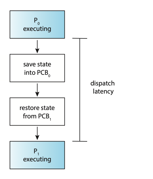
Figure: The role of the dispatcher
A voluntary context switch occurs when a process has given up contol of the CPU because it requires a resource that is currently unavailable. A non-voluntary context switch occurs when the CPU has been taken away from a process. This can occur when its time slice has expired, its been preempted by a higher-priority process, and more.
Using the /proc file system, the number of context switches for a given process
can be detemined. For example, the contents of the file /proc/2166/status provides
the following trimmed output:
voluntary_ctxt_switches       150
nonvoluntary_ctxt_swtiches    8
The Linux command vmstat can also be used to see the number of context switches
on a system-wide level.
Scheduling Criteria
Different CPU scheduling algorithms have diffeernt properties and the choice of a particular algorithm may favour one class of process over another.
Many critera have been suggested for comparing CPU scheduling alogrithms:
- CPU utilisation: We want to keep the CPU as busy as possible. Conceptually, CPU utilization can range from 0 to 100 percent. In a real system, it should range from 40 percent (for a lightly loaded system) to 90 percent (for a heavily loaded system).
- Throughput: If the CPU is busy executing processes, then work is being done. One measure of work is the number of processes that are completed per time unit, called throughput.
- Turn-around time: From the point of view of a particular process, the important criterion is how long it takes to execute that process. The interval from the time of submission of a process to the time of completion is the turnaround time. Turnaround time is the sum of the periods spent waiting in the ready queue, executing on the CPU, and doing I/O.
- Waiting time: The CPU scheduling algorithm does not affect the amount of time during which a process executes or does I/O. It only affects the amount of time that a process spends waiting in the ready queue. Waiting time is the sum of the periods spent waiting in the ready queue.
- Response time: In an interactive system, turnaround time may not be the best criterion. Often, a process can produce some output fairly early and can continue computing new results while previous results are being output to the user. Thus, another measure is the time from the submission of a request until the first response is produced. This measure, called response time, is the time it takes to start responding, not the time it takes to output the response.
In general, it is desirable to maximise CPU utilisation and thoughput, but minimise turnaround time, waiting time, and response time. In some cases however, we may prefer to optimize the minimum or maximum values rather than the average.
CPU Scheduling Alogrithms
- First-Come, First-Served Scheduling: First-come, first-served (FCFS) scheduling is the simplest scheduling algorithm, but it can cause short processes to wait for very long processes.
- Shortest-Job-First Scheduling: Shortest-job-first (SJF) scheduling is provably optimal, providing the shortest average waiting time. Implementing SJF scheduling is difficult, how- ever, because predicting the length of the next CPU burst is difficult.
- Round-Robin Scheduling: Round-robin (RR) scheduling allocates the CPU to each process for a time quantum. If the process does not relinquish the CPU before its time quantum expires, the process is preempted, and another process is scheduled to run for a time quantum.
- Priority Scheduling: Priority scheduling assigns each process a priority, and the CPU is allocated to the process with the highest priority. Processes with the same priority can be scheduled in FCFS order or using RR scheduling.
- Multilevel Queue Scheduling: Multilevel queue scheduling partitions processes into several separate queues arranged by priority, and the scheduler executes the processes in the highest-priority queue. Different scheduling algorithms may be used in each queue.
- Multilevel Feedback Queue Scheduling: Multilevel feedback queues are similar to multilevel queues, except that a process may migrate between different queues.
Thread Scheduling
On systems implementing the many-to-one and many-to-many models for thread management, the thread library schedules user-level threads to run on an available lightweight process (LPW). This scheme is known as process-contention scope (PCS) as competition for the CPU takes place among threads belonging to the same process. To determine which kernel-level thread to schedule onto a CPU, the kenel uses system-contention scope (SCS). Competition for the CPU with SCS scheduling takes place among all threads in the system. Systems that use the one-to-one model schedule threads use only SCS.
Typically, PCS is done according to priority. User-level thread priorities are set by the programmer and are not adjusted by the thread libray. PCS will typically preempt the thread currently running in favor of a higher-priority thread; however, there is no guarantee of time slicing among threads of equal priority.
Pthreads identifies the following contention scope values:
PTHREAD_SCOPE_PROCESSschedules threads using PCS scheduling.PTHREAD_SCOPE_SYSTEMschedules threads using SCS scheduling.
On systems implementing the many-to-many model, the PTHREAD_SCOPE_PROCESS policy
schedules user-level threads onto available LWPs. The PTHREAD_SCOPE_SYSTEM
scheduling policy will create and bind an LWP for each user-level thread on
many-to-many systems. This effectively maps threads using the one-to-one policy.
The Pthread IPC provides two functions for setting and getting the contention scope policy:
pthread_attr_setscope(pthread_attr_t *attr, int scope)pthread_attr_getscope(pthread_attr_t *attr, int *scope)
Below is an example program that will first determine the existing contention
scope and set it to PTHREAD_SCOPE_SYSTEM. It will then create five separate
threads that will run using the SCS scheduling policy. It's important to note
that on some systems, only certain contention scope values are allowed, i.e.
Linux and macOS only allow PTHREAD_SCOPE_SYSTEM.
#include <pthread.h>
#include <stdio.h>

#define NUM_THREADS 5

void *runner(void *param);

int main(void) {
    int scope;
    pthread_t tid[NUM_THREADS];
    pthread_attr_t attr;

    pthread_attr_init(&attr);

    if (pthread_attr_getscope(&attr, &scope) != 0) {
        fprintf(stderr, "[Error] - Unable to get scheduling scope.\n");
    } else {
        if (scope == PTHREAD_SCOPE_PROCESS) {
            printf("PTHREAD_SCOPE_PROCESS\n");
        } else if (scope == PTHREAD_SCOPE_SYSTEM) {
            printf("PTHREAD_SCOPE_SYSTEM\n");
        } else {
            fprintf(stderr, "[Error] - Illegal scope value.\n");
        }
    }

    pthread_attr_setscope(&attr, PTHREAD_SCOPE_SYSTEM);

    for (size_t i = 0; i < NUM_THREADS; i++) {
        pthread_create(&tid[i], &attr, runner, NULL);
    }

    for (size_t i = 0; i < NUM_THREADS; i++) {
        pthread_join(tid[i], NULL);
    }
}

void *runner(void *param) {
    // Do some work

    pthread_exit(0);
}
Multi-Processor Scheduling
If multiple CPUs are available, load sharing, where multiple threads may run in parallel, becomes possible, however scheduling issues become correspondingly more complex.
Traditionally, the term multiprocessor reffered to systems that provided multiple physical processors. However, the definition of multiprocessor now applies to the following system architectures:
- Multicore CPUs
- Multithreaded cores
- NUMA systems
- Hetorogeneous multiprocessing
One approach to CPU scheduling in a multiprocessor system has all scheduling decisions, I/O processing, and other system activites handled by a single processor called the master server. The other processors execute only user code. This asymmetric multiprocessing is simple because only one core accesses the system data structures, reducing the need for data sharing. The downfall for this approach however is that the master server becomes a potential bottleneck.
The standard approach for supporting multiprocessors is symmetrical multiprocessing (SMP), where each processor is self-scheduling. The scheduler for each process examines the ready queue and selects a thread to run. This provides two possible strategies for organising the threads eligible to be scheduled:
- All threads may be in a common ready queue.
- Each process may have its own private queue of threads.
Figure: Organisation of ready queues.
If option one is chosen, a possible race condition on the shared ready queue could occur and therefore must ensure that two spearate processors do not choose to schedule the same thread and that threads are not lost from the queue. To get around this, locking could be used to protect the common ready queue. This is not a great solution however, as all access to the queue would require lock ownership therefore accessing the shared queue would likely be a performance bottleneck.
The second option permits each processor to schedule threads from its private run queue. This is the most common approach on systems supporting SMP as it does not suffer from the possible performance problems associated with a shared run queue. There are possible issues with per-processor run queues such as workloads of varying size. This however, can be solved with balancing algorithms which equalise workloads among all processors.
Multicore Processors
Traditionally, SMP systems have allowed several processes to run in parallel by providing multiple physical processors. However, most contempory computer hardware now places multiple computing cores on the same physical chip resulting in a multicore processor. SMP systems that use multicore processors are faster and consume less power than systems in which each CPU has its own physical chip.
Multicore processors however, may complicate scheduling issues. When a processor accesses memory, it spends a significant amount of time waiting for the data to become available. This is known as a memory stall and occurs primarily because modern processors operate at much faster speeds than memory. A memory stall can also occur because of a cache miss, the accessing of data that is not in cache memory.
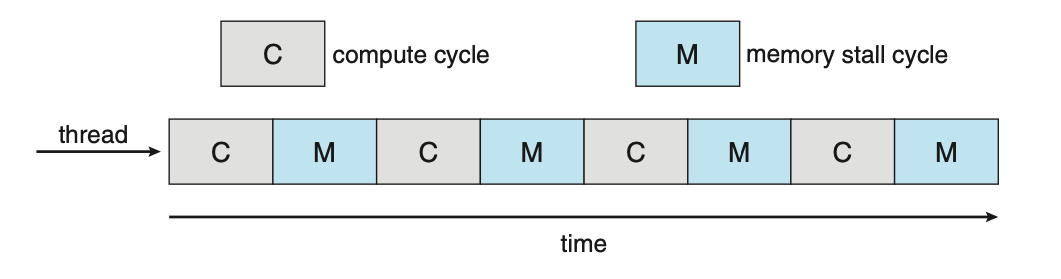
Figure: Memory stall.
To remedy this, many recent hardware designs have implemented multithreading processing cores in which two, or more, hardware threads are assigned to each core. If one hardware thread stalls, the core can switch to another thread.
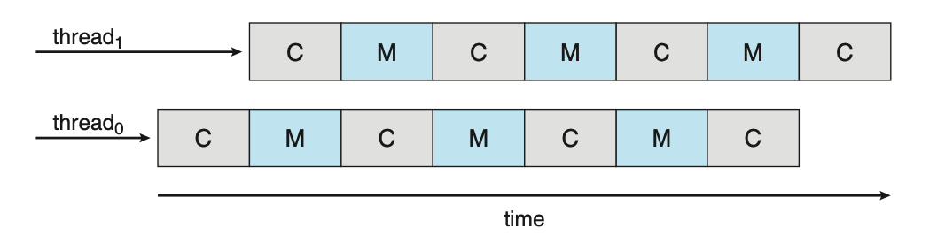
Figure: Multithreaded multicore system.
From an operating systems perspective, each hardware thread maintains its architectural state thus appearing as a logical CPU. This is known as chip multithreading (CMT). Intel processors use the term hyper-threading, or simultaneous multithreading, to describe assigning multiple hardware threads to a single processing core.
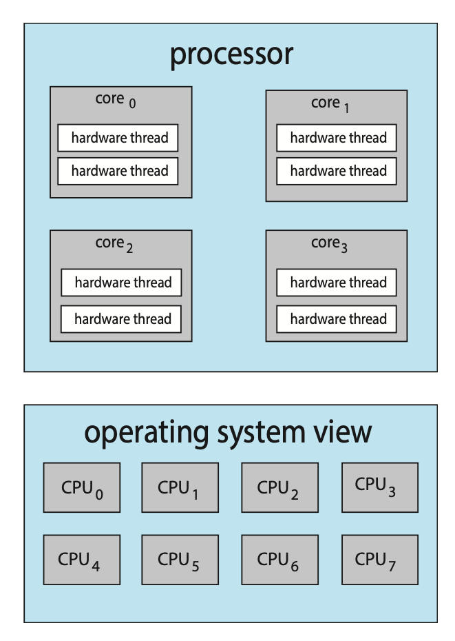
Figure: Chip multithreading.
In the above diagram, the processor contains four computing cores, each containing two hardware threads. From the perspective of the operating system, there are eight logical CPUs.
There are two ways to multithread a processing core:
- Coarse-grained multithreading
- Fine-grained multithreading
With coarse-grained multithreading, a thread executes on a core until a long-latency event occurs. Due to the delay caused by the long-latency event, the core must switch to another thread to begin execution, this is expensive. Fine-grained multithreading switches between threads at a much finer level of granularity. The architectural design of fine-grained systems includes logic for thread switching resulting in a low cost for switching between threads.
A multithreaded, multicore processor requires two different levels of scheduling. This is because the resources of the physical cores must be shared among its hardware threads and can therefore only execute one hardware thread at a time. On one level are the scheduling decisions that must be made by the operating system as it chooses which software thread to run on each hardware thread. A second level of scheduling specifies how each core decides which hardware thread to run. These two levels are not necessarily mutally exclusive.
Load Balancing
Load balancing attempts to keep the workload evenly distributed across all processors in an SMP system. Load balancing is typically necessary only on systems where each processor has its own private ready queue. On systems with a common run queue, one a processor becomes idle, it immediately extracts a runnable thread from the common ready queue.
There are two general approaches to load balancing:
- Push migration: A specific task periodically checks the load on each processor and, if it finds an imbalance, evenly distributes the load by moving (or pushing) threads from the overloaded to idle or less-busy processors.
- Pull migration: A pull migration occurs when an idle processor pulls a waiting task from a busy processor.
The concept of a balanced load may have different meanings. One view may be that a balanced load requires that all queues have approximately the same number of threads while another view may be that there must be an equal distribution of thread priorities across all queues.
Processor Affinity
As a thread runs on a specific processor, the data it uses populates the processors cache. If the thread is required to migrate to another process, the contents of the cached memory must be invalidated for the first processor, and the cache for the second processor must be repopulated. This is a high cost operation and most operating systems, with the aid of SMP, try to avoid migrating a thread from one processor to another. Instead, they attempt to keep a thread running on the same processor to take advantage of the "warm" cache. This is known as processor affinity, that is, a process has an affinity for the processor on which is is currently running.
If the approach of a common ready queue is adopted, a thread may be selected for execution by any processor. Thus, if a thread is scheduled on a new processor, that processor’s cache must be repopulated. With private, per-processor ready queues, a thread is always scheduled on the same processor and can therefore benefit from the contents of a warm cache, essentially providing processor affinity for free.
Soft affinity occurs when the operating system has a policy of attempting to keep a process running on the same process but doesn't guarantee it will do so. In contrast, some systems provide system calls that support hard affinity, thereby allowing a process to specify a subset of processors on which is can run.
Real-Time CPU Scheduling
Soft real-time systems provide no guarantee as to when a critical real-time process will be scheduled. They guarantee only that the process will be given preference over non-critical processes. In a hard real-time system, a task must be serviced by its deadline; service after the deadline has expired is the same as no service at all.
Minimising Latency
Event latency is the amount of time that elapses from when an event occurs to when it's serviced. Different events have different latency requirements. For example, the latency requirement for an antilock brake system may be between 3 to 5 milliseconds while an embedded system controlling a radar in an airliner might tolerate a latency period of several seconds.
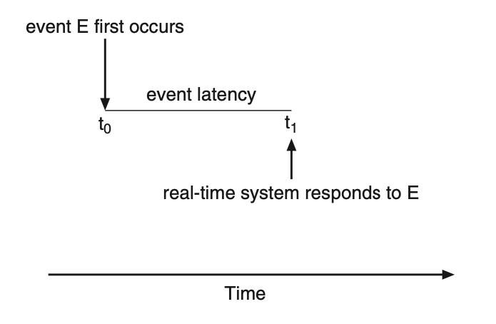
Figure: Event latency.
Two types of latencies affect the performance of real-time systems:
- Interrupt latency: The period of time from the arrival of an interrupt to the CPU to the start of the routine that services the interrupt.
- Dispatch latency: The amount of time required for the scheduling dispatcher to stop one process and start another.
Priority-Based Scheduling
TODO
Rate-Monotonic Scheduling
TODO
Earliest-Deadline-First Scheduling
TODO
Proportional Share Scheduling
TODO
POSIX Real-Time Scheduling
TODO
Week 9
Deadlocks
In a multi-programming environment, several threads may compete for a finite number of resources. A thread requests resources; if the resources are not available at that time, the thread enters a waiting state. Sometimes, a waiting thread can never again change state because the resources it has requested are heldd by other waiting threads. This is what is referred to as a deadlock.
A thread must request a resource before using it and must release the resource after using it. A thread may request as many resources as it requires to carry out its designated task. The number of resources requested may not exceed the total number of resources available in the system.
Under the normal mode of operation, a thread may utilise a resource in only the following sequence:
- Request: The thread requests the resource. If the request cannot be granted immediately, then the requesting thread must wait until it can acquire the resource.
- Use: The thread can operate on the resource.
- Release: The thread releases the resource.
The request and release of resources may be system calls such as:
request()andrelease()of a device.open()andclose()of a file.allocate()andfree()memory system calls.
Request and release can alos be accomplished through the wait()a nd signal()
operations on semaphores and through acquire() and release() of a mutex lock.
For each use of a kernel-managed resource by a thread, the operating system checks to make sure that the thread has requested and has been allocated the resource. A system table records whether each resource is free or allocated. For each resource that is allocated, the table also records the thread to which it is allocated. If a thread requests a resource that is currently allocated to another thread, it can be added to a queue of threads waiting for this resource.
// thread_one runs in this function
void *do_work_one(void *param) {
    pthread_mutex_lock(&first_mutex);
    pthread_mutex_lock(&second_mutex);

    // Do some work

    pthread_mutex_unlock(&second_mutex);
    pthread_mutex_unlock(&first_mutex);

    pthread_exit(0);
}

// thread_two runs in this function
void *do_work_two(void *param) {
    pthread_mutex_lock(&second_mutex);
    pthread_mutex_lock(&first_mutex);

    // Do some work

    pthread_mutex_unlock(&first_mutex);
    pthread_mutex_unlock(&second_mutex);

    pthread_exit(0);
}
Figure: Deadlock example.
Livelock
Livelock is another form of liveness failure. It is similar to deadlock; both prevent two or more threads from proceeding, but the threads are unable to processed for different reasons. Whereas deadlock occurs when every thread in a set is blocked waiting for an event that can be caused only by another thread in the set, livelock occurs when a thread continuously attempts an action that fails.
Livelock typically occurs when threads retry failing operations at the same time. It thus can generally be avoided by having each thread retry the failing operation at random times.
// thread_one runs in this function
void *do_work_one(void *param) {
    int done = 0;

    while (!done) {
        pthread_mutex_lock(&first_mutex);

        if (pthread_mutex_trylock(&second_mutex)) {
            // Do some work

            pthread_mutex_unlock(&second_mutex);
            pthread_mutex_unlock(&first_mutex);

            done = 1;
        } else {
            pthread_mutex_unlock(&first_mutex);
        }
    }

    pthread_exit(0);
}

// thread_two runs in this function
void *do_work_two(void *param) {
    int done = 0;

    while (!done) {
        pthread_mutex_lock(&second_mutex);

        if (pthread_mutex_trylock(&first_mutex)) {
            // Do some work

            pthread_mutex_unlock(&first_mutex);
            pthread_mutex_unlock(&second_mutex);

            done = 1;
        } else {
            pthread_mutex_unlock(&second_mutex);
        }
    }

    pthread_exit(0);
}
Figure: Livelock example.
Deadlock Charaterisation
A deadlock situation can arise if the following four conditions hold simultaneously in the system:
- Mutual exclusion: At least one resource must be held in a non-sharable mode; that is, only one thread at a time can use the resource. If another thread requests that resource, the requesting thread must be delayed until the resource has been released.
- Hold and wait: A thread must be holding at least one resource and waiting to acquire additional resources that are currently being held by other threads.
- No preemption: Resources cannot be preempted; that is, a resource can be released only voluntarily by the thread holding it, after that thread has completed its task.
- Circular wait: A set \(\{T_0, T_1, \dots, T_n\}\) of waiting threads must exist such that \(T_0\) is waiting for a resource held by \(T_1\), \(T_1\) is waiting for a resource held by \(T_2, \dots, T_{n-1}\) is waiting for a resource held by \(T_n\), and \(T_n\) is waiting for a resource held by \(T_0\).
Resource-Allocation Graph
Deadlocks can be described more precisely in terms of a directed graph called a system resource-allocation graph. The set of vertices \(V\) is partitioned into two different types of nodes:
- \(T = \{T_0, T_1, \dots, T_n\}\), the set consisting of all the active threads in the system.
- \(R = \{R_0, R_1, \dots, R_m\}\), the set consisting of all resource types in the system.
A directed edge from thread \(T_i\) to resource type \(R_j\) is denoted \(T_i \rightarrow R_j\) and is called a request edge; it signifies that thread \(T_i\) has requested an instance of resource type \(R_j\) and is currently waiting for that resource. A directed edge from resource type \(R_j\) to thread \(T_i\) is denoted \(R_j \rightarrow T_i\) and is called an assignment edge; it signifies that an instance of resource type \(R_j\) has been allocated to thread \(T_i\).
Pictorially, each thread \(T_i\) is represented as a circle and each resource type \(R_j\) as a rectangle. An instance of a resource is represented by a dot within the rectangle. For example, the below graph depicts the following situation:
- The sets \(T\), \(R\), and \(E\):
- \(T = \{T_1, T_2, T_3\}\)
- \(R = \{R_1, R_2, R_3, R_4\}\)
- \(E = \{T_1 \rightarrow R_1, T_2 \rightarrow R_3, R_1 \rightarrow T_2, R_2 \rightarrow T_2, R_2 \rightarrow T_1, R_3 \rightarrow T_3\}\)
- Resource instances:
- One instance of resource type \(R_1\)
- Two instances of resource type \(R_2\)
- One instance of resource type \(R_3\)
- Three instances of resource type \(R_4\)
- Thread states:
- Thread \(T_1\) is holding an instance of resource type \(R_2\) and is waiting for an instance of resource type \(R_1\).
- Thread \(T_2\) is holding an instance of resource type \(R_1\) and an instance of \(R_2\) and is waiting for an instance of resource type \(R_3\).
- Thread \(T_3\) is holding an instance of resource type \(R_3\).
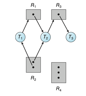
Given the definition of a resource-allocation graph, it can be shown that, if the graph contains no cycles, then no thread in the system is deadlocked. If the graph does contain a cycle, then a deadlock may exist.
- If each resource type has exactly one instance, then a cycle implies that a deadlock has occurred.
- If the cycle involves only a set of resource types, each of which has only a single instance, then a deadlock has occurred. In this case, a cycle in the graph is both a necessary and sufficient condition for the existence of deadlock.
- If each resource type has several instances, then a cycle does not necessarily imply that a deadlock has occurred. In this case, a cycle in the graph is a necessary but not a sufficient condition for the existence of deadlock.
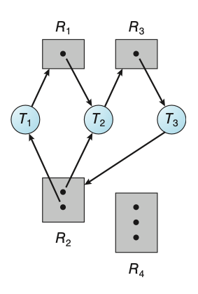
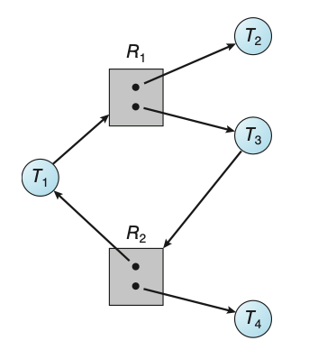
If a resource-allocation graph does not have a cycle, then the system is not in a deadlocked state. If there is a cycle, then the system may or may not be in a deadlocked state.
Methods for Handling Deadlocks
A deadlock problem can generally be dealt with in one of three ways:
- We can ignore the problem altogether and pretend that deadlocks never occur in the system.
- We can use a protocol to prevent or avoid deadlocks, ensuring that the system will never enter a deadlocked state.
- We can allow the system to enter a deadlocked state, detect it, and recover.
To ensure that deadlocks never occur, the system can use either a deadlock-prevention or a deadlock-avoidance scheme. Deadlock prevention provides a set of methods to ensure that at least one of the necessary conditions cannot hold. These methods prevent deadlocks by constraining how requests for resources can be made. Deadlock avoidance requires that the operation system be given additional information in advance concerning which resources a thread will request and use during its lifetime. With this additional information, the operating system can decide for each request whether or not the thread should wait.
Deadlock Prevention
Mutual Exclusion
The mutual-exclusion condition must hold. That is, at least one resource must be nonsharable. Sharable resources do not require mutually exclusive access and thus cannot be involved in a deadlock. Read-only files are a good example of a sharable resource. If several threads attempt to open a read-only file at the same time, they can be granted simultaneous access to the file. A thread never needs to wait for a sharable resource. In general, however, we cannot prevent deadlocks by denying the mutual-exclusion condition, because some resources are intrinsically nonsharable. For example, a mutex lock cannot be simultaneously shared by several threads.
Hold and Wait
To ensure that the hold-and-wait condition never occurs in the system, we must guarantee that, whenever a thread requests a resource, it does not hold any other resources.
- One protocol that can be used requires each thread to request and be allocated all its resources before it begins execution. This is impractical for most applications due to the dynamic nature of requesting resources.
- An alternative protocol allows a thread to request resources only when it has none. A thead may request some resources and use them. Before it can request additional resources, it must release all the resources that it is currently allocated.
Both these protocols have two main disadvantages:
- Resource utilisation may be low since resources may be allocated but unused for a long period.
- Starvation is possible. A thread that needs several popular resources may have to wait indefinitely because at least one of the resources that it needs is always allocated to some other thread.
No Preemption
The third necessary condition for deadlocks is that there be no preemption of resources that have already been allocated. To ensure that this condition does not hold, we can use the following protocol. If a thread is holding some resources and requests another resource that cannot be immediately allocated to it (that is, the thread must wait), then all resources the thread is currently holding are preempted. In other words, these resources are implicitly released. The preempted resources are added to the list of resources for which the thread is waiting. The thread will be restarted only when it can regain its old resources, as well as the new ones that it is requesting.
Alternatively, if a thread requests some resources, we first check whether they are available. If they are, we allocate them. If they are not, we check whether they are allocated to some other thread that is waiting for additional resources. If so, we preempt the desired resources from the waiting thread and allocate them to the requesting thread. If the resources are neither available nor held by a waiting thread, the requesting thread must wait. While it is waiting, some of its resources may be preempted, but only if another thread requests them. A thread can be restarted only when it is allocated the new resources it is requesting and recovers any resources that were preempted while it was waiting.
Circular Wait
One way to ensure that this condition never holds is to impose a total ordering of all resource types and to require that each thread requests resources in an increasing oredr of enumeration.
void transaction(Account from, Account to, double amount) {
    mutex lock1;
    mutex lock2;
    lock1 = get_lock(from);
    lock2 = get_lock(to);

    acquire(lock1);
        acquire(lock2);

            withdraw(from, amount);
            deposit(to, amount);

        release(lock2);
    release(lock1);
}
Deadlock Avoidance
An alternative method for avoiding deadlocks is to require additional information about how resources are to be requested. The various algorithms that use this approach differ in the amount and type of information required. The simplest and most useful model requires that each thread declare the maximum number of resources of each type that it may need. Given this prior information, it is possible to construct an algorithm that ensures that the system will never enter a deadlocked state.
Safe State
A system is in a safe state only if there exists a safe sequence. In other words, a state is safe if the system can allocate resources to each thread in some order and still avoid a deadlock. A sequence of threads \(<T_1, T_2, \dots, T_n>\) is a safe sequence for the current allocation if, for each \(T_i\), the resource requests that \(T_i\) can still make can be satisfied by the current available resources plus the resources held by all \(T_j\), with \(j < i\). If no such sequence exists, then the system state is said to be unsafe.
A safe state is not a deadlocked state. Conversely, a deadlocked state is an unsafe state. Not all unsafe states are deadlocks however. As long as the state is safe, the operating system can avoid unsafe states.
Resource-Allocation-Graph Algorithm
TODO:
Banker's Algorithm
TODO:
Safety Algorithm
TODO:
Resource-Request Algorithm
TODO:
Deadlock Detection
If a system does not employ either a deadlock-prevention or a deadlock-avoidance algorithm, then a deadlock situation may occur. In this environment, the system may provide:
- An algorithm that examines the state ofo the system to determine whether a deadlock has occured.
- An algorithm to recover from the deadlock.
Single Instance of Each Resource Type
If all resources have only a single instance, then we can define a deadlock-detection algorithm that uses a variant of the resource-allocation graph by a wait-for graph.
This graph is obtained from the resource-allocation graph by removing the resource nodes and collapsing the appropriate edges. More precisely, an edges from \(T_i\) to \(T_j\) in a wait-for graph implies that thread \(T_i\) is waiting for thread \(T_j\) to release a resource that \(T_i\) needs. An edge \(T_i \rightarrow T_j\) exists in a wait-for graph if and only if the corresponding resource-allocation graph contains two edges \(T_i \rightarrow R_q\) and \(R_q \rightarrow T_i\) for some resource \(R_q\).
As before, a deadlock exists in the system if and only if the wait-for graph contains a cycle. To detect deadlocks, the system needs to maintain the wait-for graph and periodically invoke an algorithm that searches for a cycle in the graph. An algorithm to detect a cycle in a graph requires \(O(n^2)\) operations, where \(n\) is the number of vertices in the graph.
Several Instances of a Resource Type
The wait-for graph scheme is not applicable to a resource-allocation system with multiple instances of each resource type. This algorithm employs several time-varying data structures that are similar to those used in the bankers algorithm:
- Available: A vector of length \(m\) indicates the number of available resources of each type.
- Allocation: An \(n \times m\) matrix defines the number of resources of each type currently allocated to each thread.
- Request: An \(n \times m\) matrix indicates the current request of each thread. If \(Request[i][j]\) equals \(k\), then thread \(T_i\) is requesting \(k\) more instances of resource type \(R_j\).
- Let \(Work\) and \(Finish\) be vectors of length \(m\) and \(n\), respectively. Initialise \(Work = Available\). For \(i = 0, 1, \dots, n-1\), if \(Allocation_i \ne 0\), then \(Finish[i] = false\). Otherwise, \(Finish[i] = true\).
- Find an index \(i\) such that both,
a: \(Finish[i] == false\)
b: \(Request_i \le Work\)
If no such \(i\) exists, go to step 4. - \(Work = Work + Allocation_i\)
\(Finish[i] == true\)
Go to step 2 - If \(Finish[i] == false\) for some \(i, 0 \le i \le n\), then the system is in a deadlocked state. Moreover, if \(Finish[i] == false\), then thread \(T_i\) is deadlocked.
This algorithm requires an order of \(m \times n^2\) operations to detect whether the system is in a deadlocked state.
Detection-Algorithm Usage
When should we invoke the detection algorithm? The answer depends on two factors:
- How often is a deadlock likely to occur?
- How many threads will be affected by deadlock when it happens?
If the detection algorithm is invoked at arbitrary points in time, the resource graph may contain many cycles. In this case, we generally cannot tell which of the many deadlocked threads "caused" the deadlock.
Recovery from Deadlock
When a detection algorithm determines that a deadlock exists, several alternatives are available. One possibility is to inform the operator that a deadlock has occurred and to let the operator deal with the deadlock manually. Another possibility is to let the system recover from the deadlock automatically.
There are two options for breaking a deadlock:
- Abort one or more threads to break the circular wait.
- Preempt some resources from one or more of the deadlocked threads.
Process and Thread Termination
To eliminate deadlocks by aborting a process or thread, two methods can be used. In both methods, the system reclaims all resources allocated to the terminated processes.
- Abort all deadlocked processes: This method will break the deadlock cycle, but at great expense. The deadlocked processes may have computed for a long time, and the result of these partial computations must be discarded and probably will have to be re-computed later.
- Abort one process at a time until the deadlock cycle is eliminated: This method incurs considerable overhead, since after each process is aborted, a deadlock-detection algorithm must be invoked.
Aborting a process may not be easy. If the process was in the midst of updating a file, terminating it may leave that file in an incorrect state. If the partial termination method is used, then we must determine which deadlocked process (or processes) should be terminated. This determination is a policy decision, similar to CPU-scheduling decisions. We should abort those processes whose termination will incur the minimum cost. Many factors may affect which process is chosen, such as:
- What the priority of the process is.
- How long the process has computed and how much longer the process will compute before completing its designated task.
- How many and what types of resources the process has used.
- How many more resources the process needs in order to complete.
- How many processes will need to be terminated.
Resource Preemption
To eliminate deadlocks using resource preemption, we successively preempt some resources from processes and give these resources to other processes until the deadlock cycle is broken. If preemption is required to deal with deadlocks, then three issues need to be addressed:
- Selecting a victim: Which resources and which processes are to preempted? As in process termination, we must determine the order of preemption to minimise cost.
- Rollback: If we preempt a resource from a process, what should be done with that process? Clearly, it cannot continue with its normal excecution; it is missing some needed resource. We must roll back the process to some safe state and restart it from that state. Since, in general, it is difficult to determine what a safe states is, the simplest solution is a total rollback: abort the process and then restart it.
- Starvation: How do we ensure that starvation will not occur? That is, how can we guarantee that resources will not always be preempted from the same process. In a system where victim selection is based prirmarily on cost factors, it may happen that the same process is always picked as a victim. As a result, this process never completes its designated task.
Week 11
Main Memory
Background
Memory consists of a large array of bytes, each with its own address. The CPU fetches instructions from memory according to the value of the program counter. These instructions may cause additional loading from and storing to specific memory addresses.
A typical instruction-execution cycle:
- First fetches an instruction from memory.
- The instruction is then decoded and may cause operands to be fetched from memory addresses.
- After the instruction has been executed on the operands, results may be stored back into memory.
The memory unit sees only a stream of memory addresses; it does not know how they are generated or what they are for.
Main memory and the registers built into each processing core are the only general-purpose storage that the CPU can access directly. Ther eare machin instructions that take memory addresses as arguments, but none that take disk addresses. Therefore, any instructions in execution, and any data being used by the instructions, must be in one of these direct-access storage devices. If the data are not in memory, they must be moved there before the CPU can operate on them.
Registers that are built into each CPU core are generally accessible within one cycle of the CPU clock. Some CPU cores can decode instructions and perform simple operations on register contents at the rate of one or more operations per clock tick. The same cannot be said of main memory, which is accessed via a transaction on the memory bus. Completing a memory access may take many cycles of the CPU clock. In such cases, the processor normally needs to stall, since it does not have the data required to complete the instruction that it is executing. This situation is intolerable because of the frequency of memory accesses. The remedy is to add fast memory (cache) between the CPU and main memory, typically on the CPU chip for fast access. To manage a cache built into the CPU, the hardware automatically speeds up memory access without any operating-system control.
For proper system operation, we must protect the operating system from access by user processes, as well as protect user processes from one another. This protection must be provided by the hardware, because the operating system doesn't usually intervene between the CPU and its memory accesses (because of the resulting performance penalty).
Base and Limit Registers
We first need to make sure that each process has a separate memory space. Separate per-process memory space protects the processes from each other and is fundamental to having multiple processes loaded in memory for concurrent execution. To separate memory spaces, we need the ability to determine the range of legal addresses that the process may access and to ensure that the process can access only these legal addresses. We can provide this protection by using two registers, usually a base and a limit.
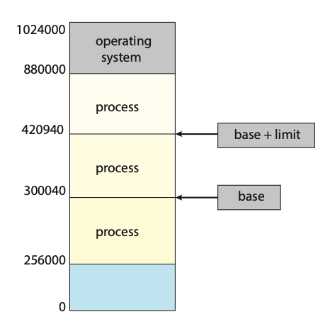
Figure: A base and a limit register define a logical address space.
The base register holds the smallest legal physical memory address; the limit register specifies the size of the range. For example, if the base register holds 300040 and the limit register is 120900, then the program can legally access all addresses from 300040 through 420939 (inclusive).
Protection of memory space is accomplished by having the CPU hardware compare every address generated in user mode with the registers. Any attempt by a program executing in user mode to access operating-system memory or other users' memory results in a trap to the operating system, which treats the attempt as a fatal error. This scheme prevents a user program from (accidentally or deliberately) modifying the code or data structures of either the operating system or other users.
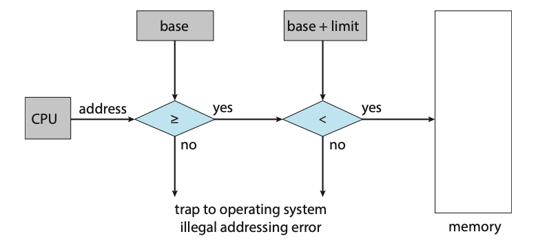 Figure: Hardware address protection with base and limit registers.
Address Binding
Usually, a program resides on a disk as a binary executable file. To run, the program must be brought into memory and placed within the context of a process, where it becomes eligible for execution on an available CPU. As the process executes, it access instructions and data from memory. Eventually, the process terminates, and its memory is reclaimed for use by other processes.
Most systems allow a user process to reside in any part of the physical memory.
Thus, although the address space of the computer may start at 00000, the first
address of the user process need not be 00000. In most cases, a user program goes
through several steps - some of which may be optional - before being executed.
Addresses may be represented in different ways during these steps. Addresses
in the source program are generally symbolic (such as the variable count). A
compiler typically binds these symbolic address to relocatable addresses (such
as "14 bytes from the beginning of this module"). The linker or loader in turn
binds the relocatable addresses to absolute addresses (such as 74014). Each binding
is a mapping from one address space to another.
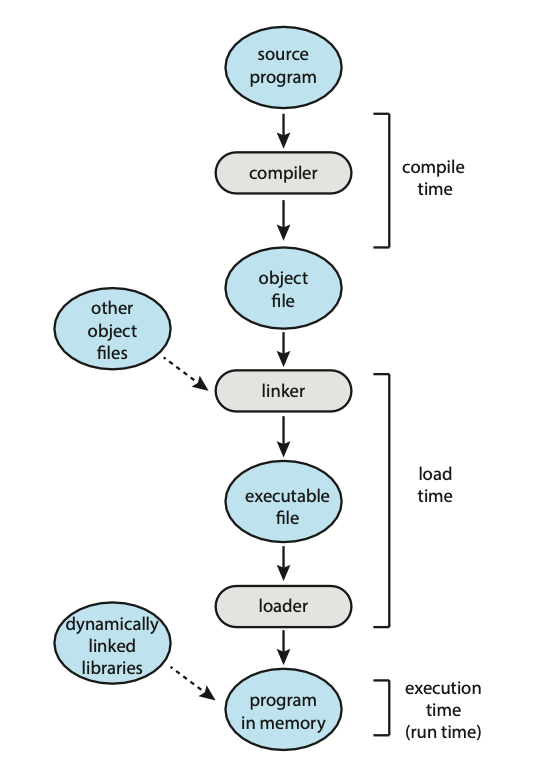 Figure: Multistep processing of a user program.
- Compile time: If you know at compile time where the process will reside in memory, then absolute code can be generated. For example, if you know that a user process will reside starting at location \(R\), then the generated compiler code will start at that location and extend up from there. If, at some later time, the starting location changes, then it will be necessary to recompile this code.
- Load time: If it is not known at compile time where the process wil reside in memory, then the compiler must generate relocatable code. In this case, final binding is delayed until load time. If the starting address changes, we need only reload the user code to incorporate this changed value.
- Execution time: If the process can be moved during its execution from one memory segment to another, then binding must be delayed until run time. Special hardware must be avaiable for this scheme to work.
Logical vs. Physical Address Space
An address generated by the CPU is commonly referred to as a logical address, whereas an address seen by the memory unit - that is, the one loaded into the memory-address register of the memory - is commonly referred to as a physical address.
Binding addresses at either compile or load time generates identical logical and physical addresses. However, the execution-time address-binding scheme results in differing logical and physical addresses. In this case, we usually refer to the logical address as a virtual address. The set of logical address generated by a program is a logical address space. The set of physical addresses corresponding to these logical addresses is a physical address space. Thus, in the execution-time address-binding scheme, the logical and physical address spaces differ.
Memory Management Unit (MMU)
THe run-time mapping from virtual to physical addresses is done by a hardware device called the memory-management unit (MMU). We can choose from many different methods to accomplish such mapping.
Consider a simple scheme where the value in the relocation register (the base register) is added to every address generated by a user process at the time it is sent to memory. For example, if the base is at 14000, then an attempt by the user to address location 0 is dynamically relocated to location 14000; an access to location 346 is mapped to location 14346.
The user program never accesses the real physical addresses. The program can create a pointer to location 346, store it in memory, manipulate it, and compare it with other addresses all as the number 346. Only when it is used as a memory address (in an indirect load or store, perhaps) is it relocated relative to the base register. The user program deals with logical addresses. The final location of a referenced memory address is not determined until the reference is made.
Dynamic Linking
So far, it has been necessary for the entire program and all data of a process to be in physical memory for the process to execute. The size of a process has thus been limited to the size of physical memory. To obtain better memory-space utilization, we can use dynamic loading. With dynamic loading, a routine is not loaded until it is called. All routines are kept on disk in a relocatable load format. The main program is loaded into memory and is executed. When a routine needs to call another routine, the calling routine first checks to see whether the other routine has been loaded. If it has not, the relocatable linking loader is called to load the desired routine into memory and to update the programs' address tables to reflect this change. Then control is passed to the newly loaded routine. Dynamic loading does not require any special support from the operating system. It is the responisiblity of the user to design their programs to take advantage of such a method. Operating systems may however help the programmer by providing library routines to implement dynamic loading.
Dynamically linked libraries (DLLs) are system libraries that are linked to user programs when the programs are run. Some operating systems support only static linking, in which system libraries are treated like any other object module and are combined by the loader into the binary program image. Dynamic linking, in contrast, is similar to dynamic loading. Here, though, linking, rather than loading, is postponed until execution time. A second advantage of DLLs is that these libraries can be shared among multiple processes, so that only one instance of the DLL is in main memory. For this reason, DLLs are also known as shared libraries.
Unlike dynamic loading, dynamic linking and shared libraries generally require help from the operating system. If the processes in memory are protected from one another, then the operating system is the only entity that can check to see whether the needed routine is in another process's memory space or that can allow multiple processes to access the same memory addresses.
Contiguous Allocation
The main memory must accommodate both the operating system and the various user procces. We therefore need to allocate main memory in the most efficient way possible. The main memory is usually divided into two partitions: one for the operating system and one for the user processes. We can place the operating system in either low memory addresses or high memory addresses. This decision depends on many factors, such as the location of the interrupt vector. However, many operating systems place the operating system in high memory.
We usually want several user processes to reside in memory at the same time. We therefore need to consider how to allocate available memory to the processes that are waiting to be brought into memory. In contiguous memory allocation, each process is contained in a single section of memory that is contiguous to the section containing the next process.
We can prevent a process from accessing memory that it does not own by combining two ideas previously discussed. If we have a system with a relocation register, together with a limit register, we accomplish our goal. The relocation register contains the value of the smallest physical address; the limit register contains the range of logical addresses. The MMU maps the logical address dynamically by adding the value in the relocation register. This mapped address is sent to memory.
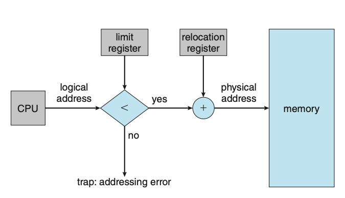
Figure: Hardware support for relocation and limit registers.
When the CPU scheduler selects a process for execution, the dispatcher loads the relocation and limit registers with the correct values as part of the context switch. Because every address generated by a CPU is checked against these registers, we can protect both the operating system and the other users’ programs and data from being modified by this running process.
One of the simplest methods of allocating memory is to assign processes to variably sized partitions in memory, where each partition may contain exactly one process. In this variable-partition shecme, the operating system keeps a table indicating which parts of memory are available and which are occupied. Initially, all memory is available for user processes and is considered one large block of available memory, a hole. Memory contains a set of holes of various sizes.
Figure: Variable partition.
Initially, the memory is fully utilised, containing processes 5, 8, and 2. After process 8 leaves, there is one contiguous hole. Later on, process 9 arrives and is allocated memory. Then process 5 departs, resulting in two non-contiguous holes.
As processes enter the system, the operating system takes into account the memory requirements of each process and the amount of availabe memory space in determining which processes are allocated memory. When a process is allocated space, it is loaded into memory, where it can then compete for CPU time. When a process terminates, it releases its memory, which the operating system may then provide to another process.
In general, the memory blocks available comprise a set of holes of various sizes scattered throughout memory. When a process arrives and needs memory, the system searches the set for a hole that is large enough for this process. If the hole is too large, it is split into two parts. One part is allocated for the arriving process; the other is returned to the set of holes. When a process terminates, it releases its block of memory, which is then placed back in the set of holes. If the new hole is adjacent to other holes, these adjacent holes are merged to form one larger hole. This procedure is a particular instance of the general dynamic storage-allocation problem, which concerns how to satisfy a request of size \(n\) from a list of free holes. There are many solutions to this problem.
- First fit: Allocate the first hole that is big enough. Searching can start either at the beginning of the set of holes or at the location where the previous first-fit search ended. We can stop searching as soon as we find a free hole that is large enough.
- Best fit: Allocate the smallest hole that is big enough. We must search the entire list, unless the list is ordered by size. This strategy produces the smallest leftover hole.
- Worst fit: Allocate the largest hole. Again, we must search the entire list, unless it is sorted by size. This strategy produces the largest leftover hole, which may be more useful than the smaller leftover hole from a best-fit approach.
Simulations have shown that both first fit and best fit are better than worst fit in terms of decreasing time and storage utilization. Neither first fit nor best fit is clearly better than the other in terms of storage utilization, but first fit is generally faster.
Fragmentation
Both the first-fit and best-fit strategies for memory allocation suffer from external fragmentation. As processes are loaded and removed from memory, the free memory space is broken into little pieces. External fragmentation exists when there is enough total memory space to satisfy a request but the available spaces are not contiguous.
Depending on the total amount of memory storage and the average process size, external fragmentation may be a minor or a major problem. Statistical analysis of first fit, for instance, reveals that, even with some optimisation, given \(N\) allocated blocks, another 0.5 \(N\) blocks will be lost to fragmentation. That is, one third of memory may be unusable. This property is known as the 50-percent rule.
Memory fragmentation can be internal as well as external. Consider a multiple-partition allocation scheme with a hole of 18,464 bytes. Suppose that the next process requests 18,462 bytes. If we allocate exactly the requested block, we are left with a hole of 2 bytes. The overhead to keep track of this hole will be substantially larger than the hole itself. The general approach to avoiding this problem is to break the physical memory into fixed-sized blocks and allocate memory in units based on block size. With this approach, the memory allocated to a process may be slightly larger than the requested memory. The difference between these two numbers is internal fragmentation — unused memory that is internal to a partition.
One solution to the problem of external fragmentation is compaction. The goal is to shuffle the memory contents so as to place all free memory together in one large block. Compaction is not always possible, however. If relocation is static and is done at assembly or load time, compaction cannot be done. It is possible only if relocation is dynamic and is done at execution time.
Paging
Paging is a memory-management scheme that permits a process's physical address space to be non-contiguous. Paging avoids external fragmentation and the associated need for compaction.
The basic method for implementing paging involves breaking physical memory into fixed-sized blocks called frames and breaking logical memory into blocks of the same size called pages. When a process is to be executed, its pages are loaded into any available memory frames from their source. The backing store is divided into fized-sized blocks that are the same size as the memory frames or clusters of multiple frames. For example, the logical address space is now totally separate from the physical address space, so a process can have a logical 64-bit address space even though the system has less than \(2^{64}\) bytes of physical memory.
Every address generated by the CPU is divided into two parts: a page numbeer (p) and a page offset (d). The page number is used as an index into a pre-process page table. The page table contains the base address of each frame in physical memory, and the offset is the location in the frame being referenced. Thus the base address of the frame is combined with the page offset to define the physical memory address.
The use of registers for the page table is satisfactory if the page table is reasonably small (for example, 256 entries). Most contemporary CPUs, however, support much larger page tables (for example, 220 entries). For these machines, the use of fast registers to implement the page table is not feasible. Rather, the page table is kept in main memory, and a page-table base register (PTBR) points to the page table. Changing page tables requires changing only this one register, substantially reducing context-switch time.
Although storing the page table in main memory can yield faster context switches, it may also result in slower memory access times. Suppose we want to access location \(i\). We must first index into the page table, using the value in the PTBR offset by the page number for \(i\). This task requires one memory access. It provides us with the frame number, which is combined with the page offset to produce the actual address. We can then access the desired place in memory. With this scheme, two memory accesses are needed to access data (one for the page-table entry and one for the actual data). Thus, memory access is slowed by a factor of 2, a delay that is considered intolerable under most circumstances.
The standard solution to this problem is to use a special, small, fast-lookup hardware cache called a translation look-aside buffer (TLB). To be able to execute the search within a pipeline step, however, the TLB must be kept small. It is typically between 32 and 1,024 entries in size. Some CPUs implement separate instruction and data address TLBs. That can double the number of TLB entries available, because those lookups occur in different pipeline steps.
If the page number is not in the TLB (known as a TLB miss), address translation proceeds, where a memory reference to the page table must be made. When the frame number is obtained, we can use it to access memory. In addition, we add the page number and frame number to the TLB, so that they will be found quickly on the next reference.
Some TLBs store address-space identifier (ASIDs) in each TLB entry. An ASID uniquely identifies each process and is used to provide address-space protection for that process. When the TLB attempts to resolve virtual page numbers, it ensures that the ASID for the currently running process matches the ASID associated with the virtual page. If the ASIDs do not match, the attempt is treated as a TLB miss. In addition to providing address-space protection, an ASID allows the TLB to contain entries for several different processes simultaneously. If the TLB does not support separate ASIDs, then every time a new page table is selected (for instance, with each context switch), the TLB must be flushed (or erased) to ensure that the next executing process does not use the wrong translation information. Otherwise, the TLB could include old entries that contain valid virtual addresses but have incorrect or invalid physical addresses left over from the previous process.
The percentage of times that the page number of interest is found in the TLB is called the hit ratio. An 80-percent hit ratio, for example, means that we find the desired page number in the TLB 80 percent of the time. If it takes 10 nanoseconds to access memory, then a mapped-memory access takes 10 nanoseconds when the page number is in the TLB. If we fail to find the page number in the TLB then we must first access memory for the page table and frame number (10 nanoseconds) and then access the desired byte in memory (10 nanoseconds), for a total of 20 nanoseconds. (We are assuming that a pagetable lookup takes only one memory access, but it can take more, as we shall see.)
To find the effective memory-access time, we weight the case by its probability:
\[ \begin{align*} \text{effective access time} &= 0.80 \times 10 + 0.20 \times 20 \\ &= 12 \text{nanoseconds} \end{align*} \]
In this example, we suffer a 20-percent slowdown in average memory-access time (from 10 to 12 nanoseconds).
Memory Protection
Memory protection in a paged environment is accomplished by protection bits associated with each frame. Normally, these bits are kept in the page table. One bit can define a page to be read - write or read-only. Every reference to memory goes through the page table to find the correct frame number. At the same time that physical address is being computed, the protection bits can be checked to verify that no writes are being made to a read-only page. At attempt to write to a read-only page causes a hardware trap to the operating system (or memory-protection violation).
One additional bit is generally attached to each entry in the page table: a valid-invalid bit. When this bit is set to valid, the associated page is in the process's logical address space and is thus a legal (or valid) page. When the bit is set to invalid, the page is not in the process's logical address space. Illegal addresses are trapped by use of the valid-invalid bit. The operating system sets this bit for each page to allow or disallow access to the page.
Rarely does a process use all its address range. In fact, many processes use only a small fraction of the address space available to them. It would be wasteful in these cases to create a page table with entries for every page in the address range. Most of this table would be unused but would take up valuable memory space. Some systems provide hardware, in the form of a page-table length register (PTLR), to indicate the size of the page table. This value is checked against every logical address to verify that the address is in the valid range for the process. Failure of this test causes an error trap to the operating system.
Shared Pages
An advantage of paging is the possibility of sharing common code, a consideration that is particularly important in an environment with multiple processes. On a typical Linux system, most user processes require the standard C library libc. One option is to have each process load its own copy of libc into its address space. If a system has 40 user processes, and the libc library is 2 MB, this would require 80 MB of memory.
If the code is reentrant code, however, it can be shared.
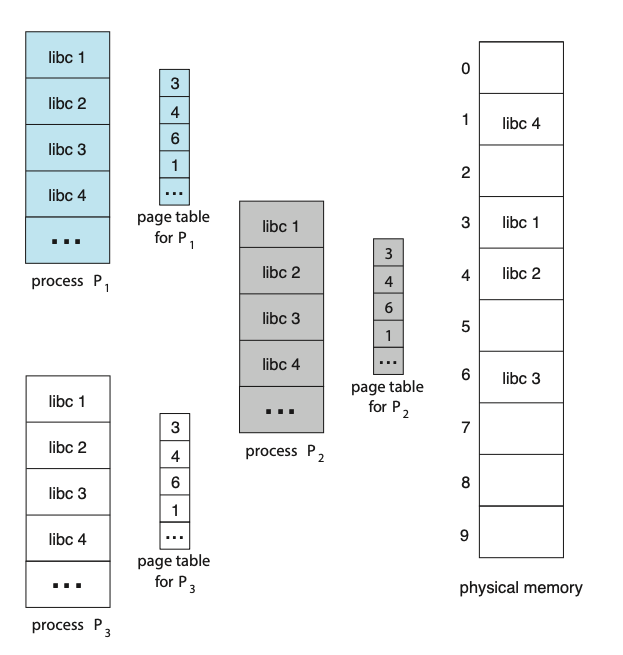
Figure: Sharing of standard C library in a paging environment.
Here, we see three processes sharing the pages for the standard C library libc. Reentrant code is non-self-modifying code: it never changes during execution. Thus, two or more processes can execute the same code at the same time. Each process has its own copy of registers and data storage to hold the data for the process’s execution. The data for two different processes will, of course, be different. Only one copy of the standard C library need be kept in physical memory, and the page table for each user process maps onto the same physical copy of libc. Thus, to support 40 processes, we need only one copy of the library, and the total space now required is 2 MB instead of 80 MB — a significant saving. In addition to run-time libraries such as libc, other heavily used programs can also be shared — compilers, window systems, database systems, and so on.
Hierarchical Page Tables
Most modern computer systems support a large logical address space (232 to 264). In such an environment, the page table itself becomes excessively large. Clearly, we would not want to allocate the page table contiguously in main memory. One simple solution to this problem is to divide the page table into smaller pieces.
One way of accomplishing this division is to use a two-level paging algorithm, in which the page table itself is also pages.
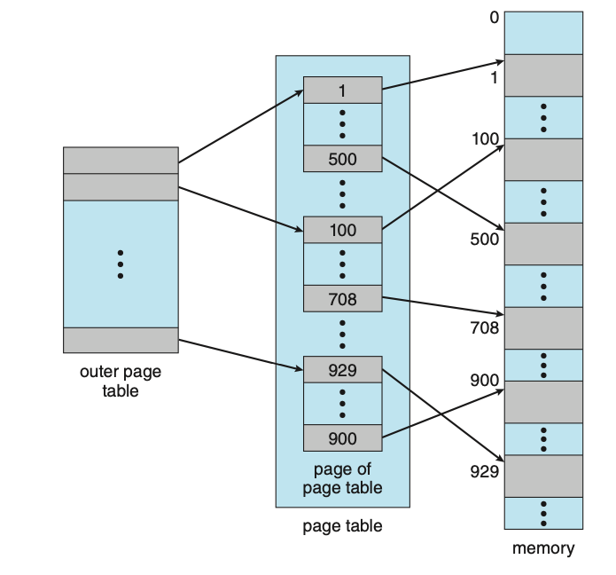
Figure: A two-level page-table scheme.
Hashed Page Tables
One approach for handling address spaces larger than 32 bits is to use a hashed page table, with the hash value being the virtual page number. Each entry in the hash table contains a linked list of elements that hash to the same location (to handle collisions). Each element consists of three fields: (1) the virtual page number, (2) the value of the mapped page frame, and (3) a pointer to the next element in the linked list.
A variation of this scheme that is useful for 64-bit address spaces has been proposed. This variation uses clustered page tables, which are similar to hashed page tables except that each entry in the hash table refers to several pages (such as 16) rather than a single page. Therefore, a single page-table entry can store the mappings for multiple physical-page frames. Clustered page tables are particularly useful for sparse address spaces, where memory references are noncontiguous and scattered throughout the address space.
Inverted Page Tables
An inverted page table has one entry for each real page (or frame) of memory. Each entry consists of the virtual address of the page stored in that real memory location, with information about the process that owns the page. Thus, only one page table is in the system, and it has only one entry for each page of physical memory.
Swapping
Process instructions and the data they operate on must be in memory to be executed. However, a process, or a portion of a process, can be swapped temporarily out of memory to a backing store and then brought back into memory for continued execution. Swapping makes it possible for the total physical address space of all processes to exceed the real physical memory of the system, thus increasing the degree of multiprogramming in a system.
Week 12
Protection
The role of protection in a computer system is to provide a mechanism for the enforcement of the policies governing resource use. These policies can be established in a variety of ways. Some are fixed in the design of the system, while others are formulated by the management of a system. Still others are defined by individual users to protect resources they “own.” A protection system, then, must have the flexibility to enforce a variety of policies.
Policies for resource use may vary by application, and they may change over time. For these reasons, protection is no longer the concern solely of the designer of an operating system. The application programmer needs to use protection mechanisms as well, to guard resources created and supported by an application subsystem against misuse.
Frequently, a guiding principle can be used throughout a project, such as the design of an operating system. Following this principle simplifies design decisions and keeps the system consistent and easy to understand. A key, timetested guiding principle for protection is the principle of least privilege. This principle dictates that programs, users, and even systems be given just enough privileges to perform their tasks.
Observing the principle of least privilege would give the system a chance to mitigate the attack — if malicious code cannot obtain root privileges, there is a chance that adequately defined permissions may block all, or at least some, of the damaging operations. In this sense, permissions can act like an immune system at the operating-system level.
Another important principle, often seen as a derivative of the principle of least privilege, is compartmentalization. Compartmentalization is the process of protecting each individual system compo- nent through the use of specific permissions and access restrictions. Then, if a component is subverted, another line of defense will “kick in” and keep the attacker from compromising the system any further.
Domain of Protection
Rings of protection separate functions into domains and order them hierarchically.
A process should be allowed to access only those objects for which it has authorization.
Furthermore, at any time, a process should be able to access only those objects
that it currently requires to complete its task. This second requirement, the
need-to-know principle, is useful in limiting the amount of damage a faulty process
or an attacker can cause in the system. For example, when process p invokes procedure
A(), the procedure should be allowed to access only its own variables and the
formal parameters passed to it; it should not be able to access all the variables
of process p.
In comparing need-to-know with least privilege, it may be easiest to think of need-to-know as the policy and least privilege as the mechanism for achieving this policy. For example, in file permissions, need-to-know might dictate that a user have read access but not write or execute access to a file. The principle of least privilege would require that the operating system provide a mechanism to allow read but not write or execute access.
To facilitate the sort of scheme just described, a process may operate within a protection domain, which specifies the resources that the process may access. Each domain defines a set of objects and the types of operations that may be invoked on each object. The ability to execute an operation on an object is an access right.
A domain is a collection of access rights, each of which is an ordered pair
<object-name, rights-set>. For example, if domain \(D\) has the access right
<file F, {read,write}>, then a process executing in domain \(D\) can both
read and write file \(F\). It cannot, however, perform any other operation on
that object.
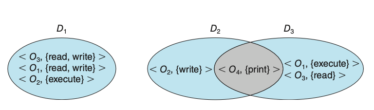
Figure: System with three protection domains.
Access Matrix
The general model of protection can be viewed abstractly as a matrix, called an
access matrix. The rows of the access matrix represent domains, and the columns
represent objects. Each entry in the matrix consists of a set of access rights.
Because the column defines objects explicitly, we can omit the object name from
the access right. The entry access(i,j) defines the set of operations that a
process executing in domain \(D_i\) can invoke on object \(O_j\).
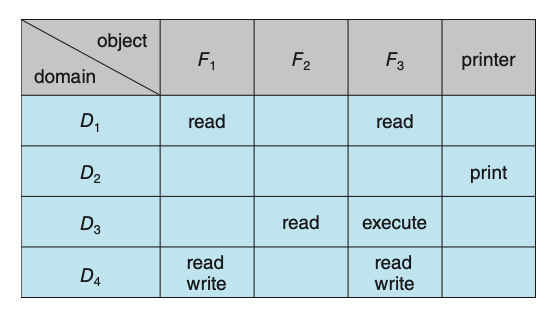
Figure: Access matrix.
When we switch a process from one domain to another, we are executing an operation (switch) on an object (the domain). Processes should be able to switch from one domain to another. Switching from domain \(D_i\) to domain \(D_j\) is allowed if and only if the access right \(\text{switch} \in \text{access}(i, j)\). Allowing controlled change in the contents of the access-matrix entries requires three additional operations: copy, owner, and control. We examine these operations next. The ability to copy an access right from one domain (or row) of the access matrix to another is denoted by an asterisk (*) appended to the access right. The copy right allows the access right to be copied only within the column (that is, for the object) for which the right is defined.
The problem of guaranteeing that no information initially held in an object can migrate outside of its execution environment is called the confinemen problem. This problem is in general unsolvable.
File Systems
Computers can store information on various storage media, such as NVM devices, HDDs, magnetic tapes, and optical disks. So that the computer system will be convenient to use, the operating system provides a uniform logical view of stored information. The operating system abstracts from the physical properties of its storage devices to define a logical storage unit, the file. Files are mapped by the operating system onto physical devices. These storage devices are usually nonvolatile, so the contents are persistent between system reboots.
A file is a named collection of related information that is recorded on secondary storage. From a user’s perspective, a file is the smallest allotment of logical secondary storage; that is, data cannot be written to secondary storage unless they are within a file. Commonly, files represent programs (both source and object forms) and data. Data files may be numeric, alphabetic, alphanumeric, or binary. Files may be free form, such as text files, or may be formatted rigidly. In general, a file is a sequence of bits, bytes, lines, or records, the meaning of which is defined by the file’s creator and user.
File Attributes
A file is named, for the convenience of its human users, and is referred to by
its name. A name is usually a string of characters, such as example.c. Some
systems differentiate between uppercase and lowercase characters in names, whereas
other systems do not. When a file is named, it becomes independent of the process,
the user, and even the system that created it. For instance, one user might create
the file example.c, and another user might edit that file by specifying its name.
The file’s owner might write the file to a USB drive, send it as an e-mail attachment,
or copy it across a network, and it could still be called example.c on the
destination system. Unless there is a sharing and synchonization method, that
second copy is now independent of the first and can be changed separately.
A file’s attributes vary from one operating system to another but typically consist of these:
- Name: The symbolic file name is the only information kept in humanreadable form.
- Identifier: This unique tag, usually a number, identifies the file within the file system; it is the non-human-readable name for the file.
- Type: This information is needed for systems that support different types of files.
- Location: This information is a pointer to a device and to the location of the file on that device.
- Size: The current size of the file (in bytes, words, or blocks) and possibly the maximum allowed size are included in this attribute.
- Protection: Access-control information determines who can do reading, writing, executing, and so on.
- Timestamps and user identification: This information may be kept for creation, last modification, and last use. These data can be useful for protection, security, and usage monitoring.
The information about all files is kept in the directory structure, which resides on the same device as the files themselves.
File Operations
A file is an abstract data type. To define a file properly, we need to consider the operations that can be performed on files. The operating system can provide system calls to create, write, read, reposition, delete, and truncate files.
- Creating a file: Two steps are necessary to create a file. First, space in the file system must be found for the file. Second, an entry for the new file must be made in a directory.
- Opening a file: Rather than have all file operations specify a file name, causing the operating system to evaluate the name, check access permissions, and so on, all operations except create and delete require a file open() first. If successful, the open call returns a file handle that is used as an argument in the other calls.
- Writing a file: To write a file, we make a system call specifying both the open file handle and the information to be written to the file. The system must keep a write pointer to the location in the file where the next write is to take place if it is sequential. The write pointer must be updated whenever a write occurs.
- Reading a file: To read from a file, we use a system call that specifies the file handle and where (in memory) the next block of the file should be put. Again, the system needs to keep a read pointer to the location in the file where the next read is to take place, if sequential. Once the read has taken place, the read pointer is updated. Because a process is usually either reading from or writing to a file, the current operation location can be kept as a per-process current-file-positio pointer. Both the read and write operations use this same pointer, saving space and reducing system complexity.
- Repositioning within a file: The current-file-position pointer of the open file is repositioned to a given value. Repositioning within a file need not involve any actual I/O. This file operation is also known as a file seek.
- Deleting a file: To delete a file, we search the directory for the named file. Having found the associated directory entry, we release all file space, so that it can be reused by other files, and erase or mark as free the directory entry. Note that some systems allow hard links—multiple names (directory entries) for the same file. In this case the actual file contents is not deleted until the last link is deleted.
- Truncating a file: The user may want to erase the contents of a file but keep its attributes. Rather than forcing the user to delete the file and then recreate it, this function allows all attributes to remain unchanged — except for file length. The file can then be reset to length zero, and its file space can be released.
Most of the file operations mentioned involve searching the directory for the
entry associated with the named file. To avoid this constant searching, many
systems require that an open() system call be made before a file is first used.
The operating system keeps a table, called the open-file table, containing information
about all open files. When a file operation is requested, the file is specified
via an index into this table, so no searching is required. When the file is no
longer being actively used, it is closed by the process, and the operating system
removes its entry from the open-file table, potentially releasing locks.
create() and delete() are system calls that work with closed rather than open
files.
Typically, the open-file table also has an open count associated with each file
to indicate how many processes have the file open. Each close() decreases this
open count, and when the open count reaches zero, the file is no longer in use,
and the file’s entry is removed from the open-file table.
Some operating systems provide facilities for locking an open file (or sections of a file). File locks allow one process to lock a file and prevent other processes from gaining access to it. File locks are useful for files that are shared by several processes - for example, a system log file that can be accessed and modified by a number of processes in the system. File locks provide functionality similar to reader–writer locks. A shared lock is akin to a reader lock in that several processes can acquire the lock concurrently. An exclusive lock behaves like a writer lock; only one process at a time can acquire such a lock.
Furthermore, operating systems may provide either mandatory or advisory file-locking
mechanisms. With mandatory locking, once a process acquires an exclusive lock,
the operating system will prevent any other process from accessing the locked file.
For example, assume a process acquires an exclusive lock on the file system.log.
If we attempt to open system.log from another process — for example, a text editor —
the operating system will prevent access until the exclusive lock is released.
Alternatively, if the lock is advisory, then the operating system will not prevent
the text editor from acquiring access to system.log. Rather, the text editor
must be written so that it manually acquires the lock before accessing the file.
In other words, if the locking scheme is mandatory, the operating system ensures
locking integrity. For advisory locking, it is up to software developers to ensure
that locks are appropriately acquired and released.
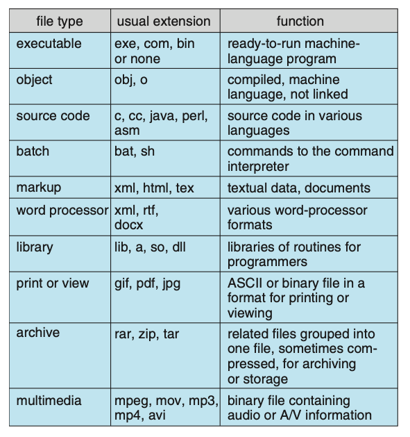
Figure: Common file types.
File Structure
Some operating systems impose (and support) a minimal number of file structures. This approach has been adopted in UNIX, Windows, and others. UNIX considers each file to be a sequence of 8-bit bytes; no interpretation of these bits is made by the operating system. This scheme provides maximum flexibility but little support. Each application program must include its own code to interpret an input file as to the appropriate structure. However, all operating systems must support at least one structure—that of an executable file—so that the system is able to load and run programs.
File types also can be used to indicate the internal structure of the file. Source and object files have structures that match the expectations of the programs that read them. Further, certain files must conform to a required structure that is understood by the operating system. For example, the operating system requires that an executable file have a specific structure so that it can determine where in memory to load the file and what the location of the first instruction is. Some operating systems extend this idea into a set of system-supported file structures, with sets of special operations for manipulating files with those structures.
Access Methods
Files store information. When it is used, this information must be accessed and read into computer memory. The information in the file can be accessed in several ways. Some systems provide only one access method for files. Others (such as mainframe operating systems) support many access methods, and choosing the right one for a particular application is a major design problem.
The simplest access method is sequential access. Information in the file is processed
in order, one record after the other. This mode of access is by far the most common;
for example, editors and compilers usually access files in this fashion. Reads
and writes make up the bulk of the operations on a file. A read operation — read_next()
— reads the next portion of the file and automatically advances a file pointer,
which tracks the I/O location. Similarly, the write operation— write_next() —
appends to the end of the file and advances to the end of the newly written
material (the new end of file). Such a file can be reset to the beginning, and
on some systems, a program may be able to skip forward or backward \(n\) records
for some integer \(n\) — perhaps only for \(n = 1\)).
Another method is direct access (or relative access). Here, a file is made up of fixed-length logical records that allow programs to read and write records rapidly in no particular order. The direct-access method is based on a disk model of a file, since disks allow random access to any file block. For direct access, the file is viewed as a numbered sequence of blocks or records. Thus, we may read block 14, then read block 53, and then write block 7. There are no restrictions on the order of reading or writing for a direct-access file. Direct-access files are of great use for immediate access to large amounts of information. Databases are often of this type. When a query concerning a particular subject arrives, we compute which block contains the answer and then read that block directly to provide the desired information.
For the direct-access method, the file operations must be modified to include
the block number as a parameter. Thus, we have read(n), where n is the block
number, rather than read next(), and write(n) rather than write next().
An alternative approach is to retain read next() and write next() and to add
an operation position file(n) where n is the block number. Then, to effect
a read(n), we would position file(n) and then read next().
The block number provided by the user to the operating system is normally a relative block number. A relative block number is an index relative to the beginning of the file. Thus, the first relative block of the file is 0, the next is 1, and so on, even though the absolute disk address may be 14703 for the first block and 3192 for the second. The use of relative block numbers allows the operating system to decide where the file should be placed (called the allocation problem) and helps to prevent the user from accessing portions of the file system that may not be part of her file.
Other Access Methods
Other access methods can be built on top of a direct-access method. These methods generally involve the construction of an index for the file. The index, like an index in the back of a book, contains pointers to the various blocks. To find a record in the file, we first search the index and then use the pointer to access the file directly and to find the desired record.
With large files, the index file itself may become too large to be kept in memory. One solution is to create an index for the index file. The primary index file contains pointers to secondary index files, which point to the actual data items.
Types of File Systems
Computer systems may also have varying numbers of file systems, and the file systems may be of varying types. Consider the types of file systems in Solaris:
- tmpfs: A “temporary” file system that is created in volatile main memory and has its contents erased if the system reboots or crashes
- objfs: A “virtual” file system (essentially an interface to the kernel that looks like a file system) that gives debuggers access to kernel symbols.
- ctfs: A virtual file system that maintains “contract” information to manage which processes start when the system boots and must continue to run during operation.
- lofs: A “loop back” file system that allows one file system to be accessed in place of another one.
- procfs: A virtual file system that presents information on all processes as a file system.
- ufs, zfs: A general-purpose file systems.
Directory Structure
The directory can be viewed as a symbol table that translates file names into their file control blocks. If we take such a view, we see that the directory itself can be organized in many ways. The organization must allow us to insert entries, to delete entries, to search for a named entry, and to list all the entries in the directory.
When considering a particular directory structure, we need to keep in mind the operations that are to be performed on a directory:
- Search for a file: We need to be able to search a directory structure to find the entry for a particular file. Since files have symbolic names, and similar names may indicate a relationship among files, we may want to be able to find all files whose names match a particular pattern.
- Create a file: New files need to be created and added to the directory.
- Delete a file: When a file is no longer needed, we want to be able to remove it from the directory. Note a delete leaves a hole in the directory structure and the file system may have a method to defragement the directory structure.
- List a directory: We need to be able to list the files in a directory and the contents of the directory entry for each file in the list.
- Rename a file: Because the name of a file represents its contents to its users, we must be able to change the name when the contents or use of the file changes. Renaming a file may also allow its position within the directory structure to be changed.
- Traverse the file system: We may wish to access every directory and every file within a directory structure. For reliability, it is a good idea to save the contents and structure of the entire file system at regular intervals. Often, we do this by copying all files to magnetic tape, other secondary storage, or across a network to another system or the cloud. This technique provides a backup copy in case of system failure. In addition, if a file is no longer in use, the file can be copied the backup target and the disk space of that file released for reuse by another file.
Single-Level Directory
The simplest directory structure is the single-level directory. All files are contained in the same directory.
- Advantages:
- Easy to implement.
- Easy to understand.
- Disadvantages:
- Since all files are in the same directory, they must have unique names.
- Relevant files cannot be grouped together.
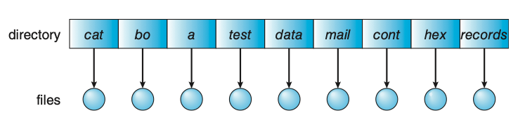
Figure: Single-level directory.
Two-Level Directory
In the two-level directory structure, each user has his own user file directory (UFD). The UFDs have similar structures, but each lists only the files of a single user. When a user refers to a particular file, only his own UFD is searched. Thus, different users may have files with the same name, as long as all the file names within each UFD are unique.
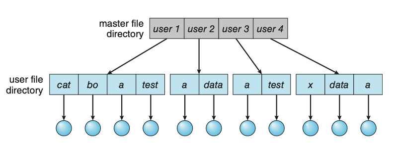
Figure: Two-level directory structure.
Tree-Structured Directories
Once we have seen how to view a two-level directory as a two-level tree, the natural generalization is to extend the directory structure to a tree of arbitrary height. This generalization allows users to create their own subdirectories and to organize their files accordingly. A tree is the most common directory structure. The tree has a root directory, and every file in the system has a unique path name. A directory (or subdirectory) contains a set of files or subdirectories. In many implementations, a directory is simply another file, but it is treated in a special way. All directories have the same internal format. One bit in each directory entry defines the entry as a file (0) or as a subdirectory (1).
Path names can be of two types: absolute and relative. In UNIX and Linux, an
absolute path name begins at the root (which is designated by an initial “/”)
and follows a path down to the specified file, giving the directory names on the
path. A relative path name defines a path from the current directory. For example
if the current directory is /spell/mail, then the relative path name prt/first
refers to the same file as does the absolute path name /spell/mail/prt/first.
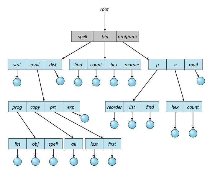
Figure: Tree-structured directory structure.
Acyclic-Graph Directories
Consider two programmers who are working on a joint project. The files associated with that project can be stored in a subdirectory, separating them from other projects and files of the two programmers. But since both programmers are equally responsible for the project, both want the subdirectory to be in their own directories. In this situation, the common subdirectory should be shared. A shared directory or file exists in the file system in two (or more) places at once.
A tree structure prohibits the sharing of files or directories. An acyclic graph — that is, a graph with no cycles — allows directories to share subdirectories and files. The same file or subdirectory may be in two different directories. The acyclic graph is a natural generalization of the tree-structured directory scheme.
Shared files and subdirectories can be implemented in several ways. A common way, exemplified by UNIX systems, is to create a new directory entry called a link. A link is effectively a pointer to another file or subdirectory. For example, a link may be implemented as an absolute or a relative path name. When a reference to a file is made, we search the directory. If the directory entry is marked as a link, then the name of the real file is included in the link information. We resolve the link by using that path name to locate the real file. Links are easily identified by their format in the directory entry (or by having a special type on systems that support types) and are effectively indirect pointers. The operating system ignores these links when traversing directory trees to preserve the acyclic structure of the system.
Figure: Acyclic-graph directory structure.
File System Mounting
Just as a file must be opened before it can be used, a file system must be mounted before it can be available to processes on the system. More specifically, the directory structure may be built out of multiple file-system-containing volumes, which must be mounted to make them available within the file- system name space.
The mount procedure is straightforward. The operating system is given the name of the device and the mount point — the location within the file structure where the file system is to be attached. Some operating systems require that a file-system type be provided, while others inspect the structures of the device and determine the type of file system. Typically, a mount point is an empty directory.
Disk Structure
- Disk can be subdivided into partitions. Disks or partitions can be RAID (Redundant Array of Independent Disks) protected against failure.
- Disk or partition can be used raw – without a file system, or formatted with a file system.
- A disk can be sliced into multiple partitions, or a volume can span multiple partitions on multiple disks.
- An entity containing a file system known as a volume. Each volume containing file system also tracks that file system’s info in a device directory or volume table of contents.
- As well as general-purpose file systems there are many special-purpose file systems, frequently all within the same operating system or computer.
Week 13
Virtual Machines
The fundamental idea behind a virtual machine is to abstract the hardware of a single computer (the CPU, memory, disk drives, network interface cards, and so forth) into several different execution environments, thereby creating the illusion that each separate environment is running on its own private computer. This concept may seem similar to the layered approach of operating system implementation, and in some ways it is. In the case of virtualization, there is a layer that creates a virtual system on which operating systems or applications can run.
Virtual machine implementations involve several components. At the base is the host, the underlying hardware system that runs the virtual machines. The virtual machine manager (VMM) (also known as a hypervisor) creates and runs virtual machines by providing an interface that is identical to the host (except in the case of paravirtualization). Each guest process is provided with a virtual copy of the host. Usually, the guest process is in fact an operating system. A single physical machine can thus run multiple operating systems concurrently, each in its own virtual machine.
Figure: System models. (a) Nonvirtual machine. (b) Virtual machine.
Types of Hypervisors
The implementation of VMMs varies greatly. Options include the following:
- Hardware-based solutions that provide support for virtual machine creation and management via firmware. These VMMs, which are commonly found in mainframe and large to midsized servers, are generally known as type 0 hypervisors. IBM LPARs and Oracle LDOMs are examples.
- Operating-system-like software built to provide virtualization, including VMware ESX (mentioned above), Joyent SmartOS, and Citrix XenServer. These VMMs are known as type 1 hypervisors.
- Applications that run on standard operating systems but provide VMM features to guest operating systems. These applications, which include VMware Workstation and Fusion, Parallels Desktop, and Oracle Virtual- Box, are type 2 hypervisors.
Benefits and Features
Several advantages make virtualization attractive. Most of them are fundamentally related to the ability to share the same hardware yet run several different execution environments (that is, different operating systems) concurrently.
One important advantage of virtualization is that the host system is protected from the virtual machines, just as the virtual machines are protected from each other. A virus inside a guest operating system might damage that operating system but is unlikely to affect the host or the other guests. Because each virtual machine is almost completely isolated from all other virtual machines, there are almost no protection problems.
One feature common to most virtualization implementations is the ability to freeze, or suspend, a running virtual machine. Many operating systems provide that basic feature for processes, but VMMs go one step further and allow copies and snapshots to be made of the guest. The copy can be used to create a new VM or to move a VM from one machine to another with its current state intact. The guest can then resume where it was, as if on its original machine, creating a clone. The snapshot records a point in time, and the guest can be reset to that point if necessary (for example, if a change was made but is no longer wanted).
A virtual machine system is a perfect vehicle for operating-system research and development. Normally, changing an operating system is a difficult task. Operating systems are large and complex programs, and a change in one part may cause obscure bugs to appear in some other part. The power of the operating system makes changing it particularly dangerous. Because the operating system executes in kernel mode, a wrong change in a pointer could cause an error that would destroy the entire file system. Thus, it is necessary to test all changes to the operating system carefully.
Another advantage of virtual machines for developers is that multiple operating systems can run concurrently on the developer’s workstation. This virtualized workstation allows for rapid porting and testing of programs in varying environments. In addition, multiple versions of a program can run, each in its own isolated operating system, within one system. Similarly, quality assurance engineers can test their applications in multiple environments without buying, powering, and maintaining a computer for each environment.
A major advantage of virtual machines in production data-center use is system consolidation, which involves taking two or more separate systems and running them in virtual machines on one system. Such physical-to-virtual conversions result in resource optimization, since many lightly used systems can be combined to create one more heavily used system.
Consider, too, that management tools that are part of the VMM allow system administrators to manage many more systems than they otherwise could. A virtual environment might include 100 physical servers, each running 20 virtual servers. Without virtualization, 2,000 servers would require several system administrators. With virtualization and its tools, the same work can be managed by one or two administrators. One of the tools that make this possible is templating, in which one standard virtual machine image, including an installed and configured guest operating system and applications, is saved and used as a source for multiple running VMs. Other features include managing the patching of all guests, backing up and restoring the guests, and monitoring their resource use.
Virtualization can improve not only resource utilization but also resource management. Some VMMs include a live migration feature that moves a run- ning guest from one physical server to another without interrupting its opera- tion or active network connections. If a server is overloaded, live migration can thus free resources on the source host while not disrupting the guest. Similarly, when host hardware must be repaired or upgraded, guests can be migrated to other servers, the evacuated host can be maintained, and then the guests can be migrated back. This operation occurs without downtime and without interruption to users.
Types of VMs
Whatever the hypervisor type, at the time a virtual machine is created, its creator gives the VMM certain parameters. These parameters usually include the number of CPUs, amount of memory, networking details, and storage details that the VMM will take into account when creating the guest. For example, a user might want to create a new guest with two virtual CPUs, 4 GB of memory, 10 GB of disk space, one network interface that gets its IP address via DHCP, and access to the DVD drive.
The VMM then creates the virtual machine with those parameters. In the case of a type 0 hypervisor, the resources are usually dedicated. In this situation, if there are not two virtual CPUs available and unallocated, the creation request in our example will fail. For other hypervisor types, the resources are dedicated or virtualized, depending on the type. Certainly, an IP address cannot be shared, but the virtual CPUs are usually multiplexed on the physical CPUs. Similarly, memory management usually involves allocating more memory to guests than actually exists in physical memory. Finally, when the virtual machine is no longer needed, it can be deleted. When this happens, the VMM first frees up any used disk space and then removes the configuration associated with the virtual machine, essentially forgetting the virtual machine.
This ease of creation can lead to virtual machine sprawl, which occurs when there are so many virtual machines on a system that their use, history, and state become confusing and difficult to track.
Type 0 Hypervisor
Type 0 hypervisors have existed for many years under many names, including “partitions” and “domains.” They are a hardware feature, and that brings its own positives and negatives. Operating systems need do nothing special to take advantage of their features. The VMM itself is encoded in the firmware and loaded at boot time. In turn, it loads the guest images to run in each partition. The feature set of a type 0 hypervisor tends to be smaller than those of the other types because it is implemented in hardware. For example, a system might be split into four virtual systems, each with dedicated CPUs, memory, and I/O devices. Each guest believes that it has dedicated hardware because it does, simplifying many implementation details.
I/O presents some difficulty, because it is not easy to dedicate I/O devices to guests if there are not enough. What if a system has two Ethernet ports and more than two guests, for example? Either all guests must get their own I/O devices, or the system must provided I/O device sharing. In these cases, the hypervisor manages shared access or grants all devices to a control partition. In the control partition, a guest operating system provides services (such as networking) via daemons to other guests, and the hypervisor routes I/O requests appropriately. Some type 0 hypervisors are even more sophisticated and can move physical CPUs and memory between running guests. In these cases, the guests are paravirtualized, aware of the virtualization and assisting in its execution.
Because type 0 virtualization is very close to raw hardware execution, it should be considered separately from the other methods discussed here. A type 0 hypervisor can run multiple guest operating systems (one in each hardware partition). All of those guests, because they are running on raw hardware, can in turn be VMMs. Essentially, each guest operating system in a type 0 hypervisor is a native operating system with a subset of hardware made available to it. Because of that, each can have its own guest operating systems. Other types of hypervisors usually cannot provide this virtualization-within- virtualization functionality.
Figure: Type 0 hypervisor.
Type 1 Hypervisor
Type 1 hypervisors are commonly found in company data centers and are, in a sense, becoming “the data-center operating system.” They are special-purpose operating systems that run natively on the hardware, but rather than providing system calls and other interfaces for running programs, they create, run, and manage guest operating systems. In addition to running on standard hard- ware, they can run on type 0 hypervisors, but not on other type 1 hypervisors. Whatever the platform, guests generally do not know they are running on anything but the native hardware.
Type 1 hypervisors run in kernel mode, taking advantage of hardware protection. Where the host CPU allows, they use multiple modes to give guest operating systems their own control and improved performance. They implement device drivers for the hardware they run on, since no other component could do so. Because they are operating systems, they must also provide CPU scheduling, memory management, I/O management, protection, and even security.
By using type 1 hypervisors, data-center managers can control and manage the operating systems and applications in new and sophisticated ways. An important benefit is the ability to consolidate more operating systems and applications onto fewer systems. For example, rather than having ten systems running at 10 percent utilization each, a data center might have one server man- age the entire load. If utilization increases, guests and their applications can be moved to less-loaded systems live, without interruption of service.
Another type of type 1 hypervisor includes various general-purpose operating systems with VMM functionality. Here, an operating system such as RedHat Enterprise Linux, Windows, or Oracle Solaris performs its normal duties as well as providing a VMM allowing other operating systems to run as guests. Because of their extra duties, these hypervisors typically provide fewer virtual- ization features than other type 1 hypervisors. In many ways, they treat a guest operating system as just another process, but they provide special handling when the guest tries to execute special instructions.
Type 2 Hypervisor
This type of VMM is simply another process run and managed by the host, and even the host does not know that virtual- ization is happening within the VMM. Type 2 hypervisors have limits not associated with some of the other types. For example, a user needs administrative privileges to access many of the hardware assistance features of modern CPUs. If the VMM is being run by a standard user without additional privileges, the VMM cannot take advantage of these features. Due to this limitation, as well as the extra overhead of running a general-purpose operating system as well as guest operating systems, type 2 hypervisors tend to have poorer overall performance than type 0 or type 1.
As is often the case, the limitations of type 2 hypervisors also provide some benefits. They run on a variety of general-purpose operating systems, and running them requires no changes to the host operating system. A student can use a type 2 hypervisor, for example, to test a non-native operating system without replacing the native operating system. In fact, on an Apple laptop, a student could have versions of Windows, Linux, Unix, and less common operating systems all available for learning and experimentation.
Live Migration
One feature not found in general-purpose operating systems but found in type 0 and type 1 hypervisors is the live migration of a running guest from one system to another. A running guest on one system is copied to another system running the same VMM. The copy occurs with so little interruption of service that users logged in to the guest, as well as network connections to the guest, continue without noticeable impact. This rather astonishing ability is very powerful in resource management and hardware administration.
Figure: Live migration of a guest between two servers.
Energy Efficiency
Data centres consume a huge amount of energy resulting in high operational costs and carbon dioxide emissions. It's estimated that the energy consumption by data centres worldwide comprises about 1.3% of the global energy usage; The energy consumption by data centres in Australia is about 1.5% of Australian’s total energy consumption.
At this scale, even relatively modest energy efficiency improvements in data centers yield significant savings in operational costs and avert millions of tons of carbon dioxide emissions. Reducing the energy consumption of the IT equipment is more important than reducing the energy consumption of the non-IT equipment. When the energy consumption of the IT equipment decreases by 1 watt, the energy consumed by the non-IT equipment will decrease by 1.7 - 2.3 watts.
The server consolidation problem can be modelled as a Virtual Machine Placement (VMP) problem. Given the CPU and memory capacities of the PMs in a data centre, the CPU and memory requirements of each of the VMs in the data centre, the physical communication topology of the PMs, the VMP is to find a placement of the VMs on the PMs such that the total energy consumption of the PMs which are hosting at least one VM is minimised, subject to:
- The total CPU requirement of the VMs placed on any PM does not exceed the CPU capacity of the PM; and
- The total memory requirement of the VMs placed on any PM does not exceed the memory capacity of the PM.